Rのプロットパラメータについて
未完成ですが、とりあえず。
Test data
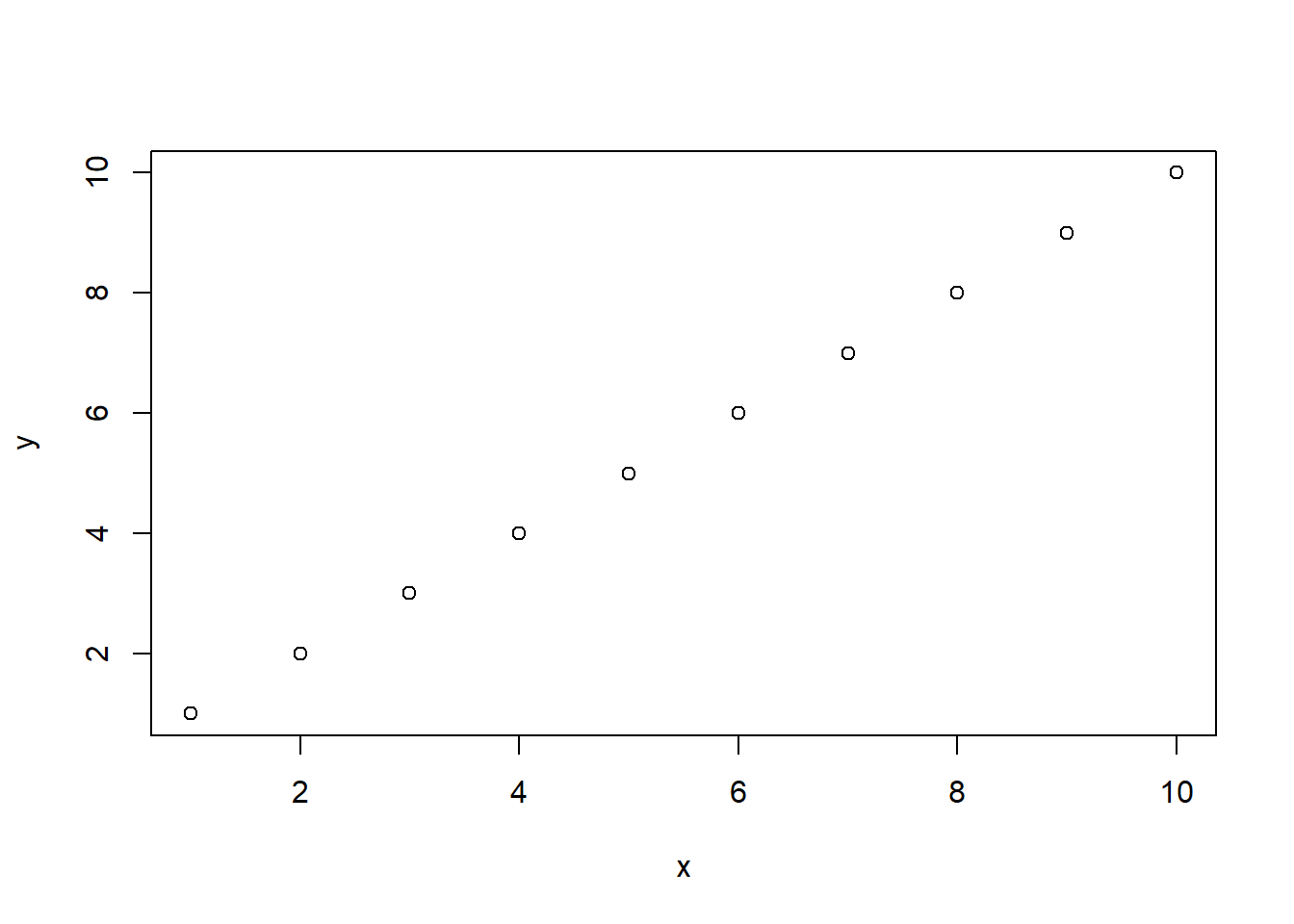
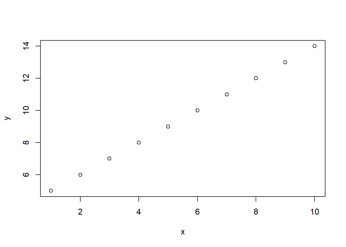
Normal scatter plot
通常の散布図
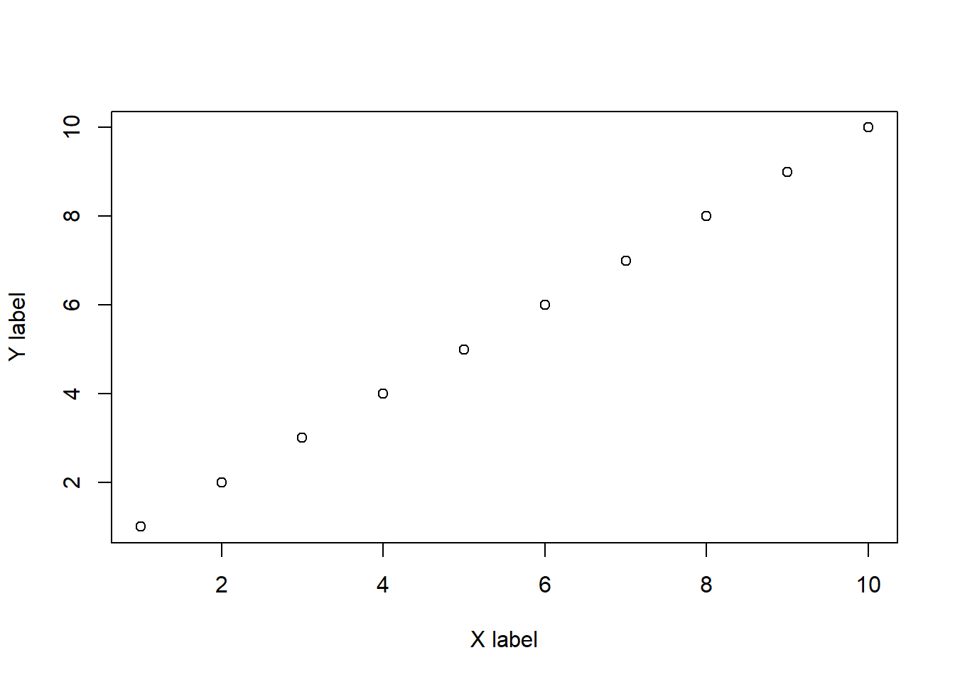
Title and label
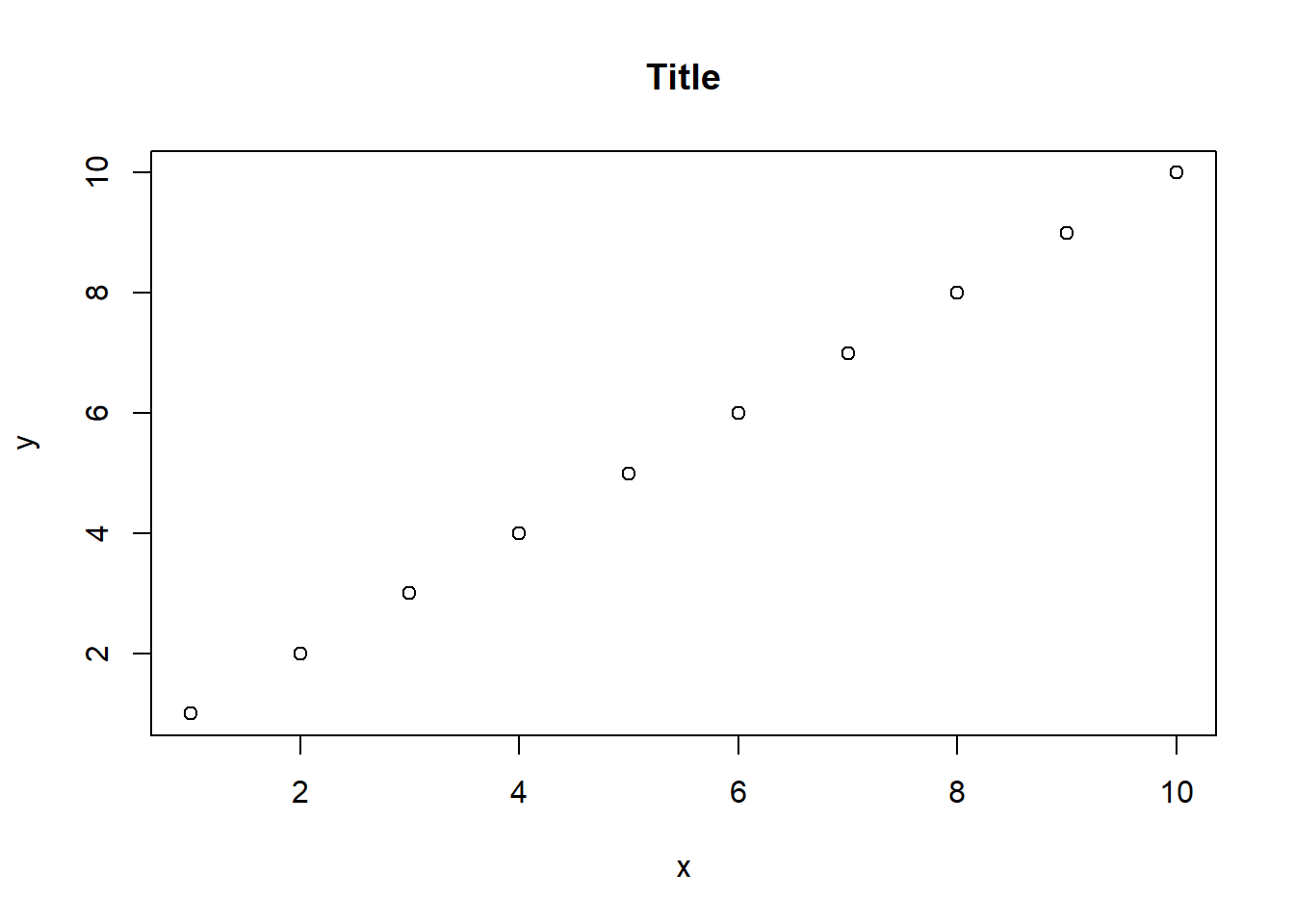
Title
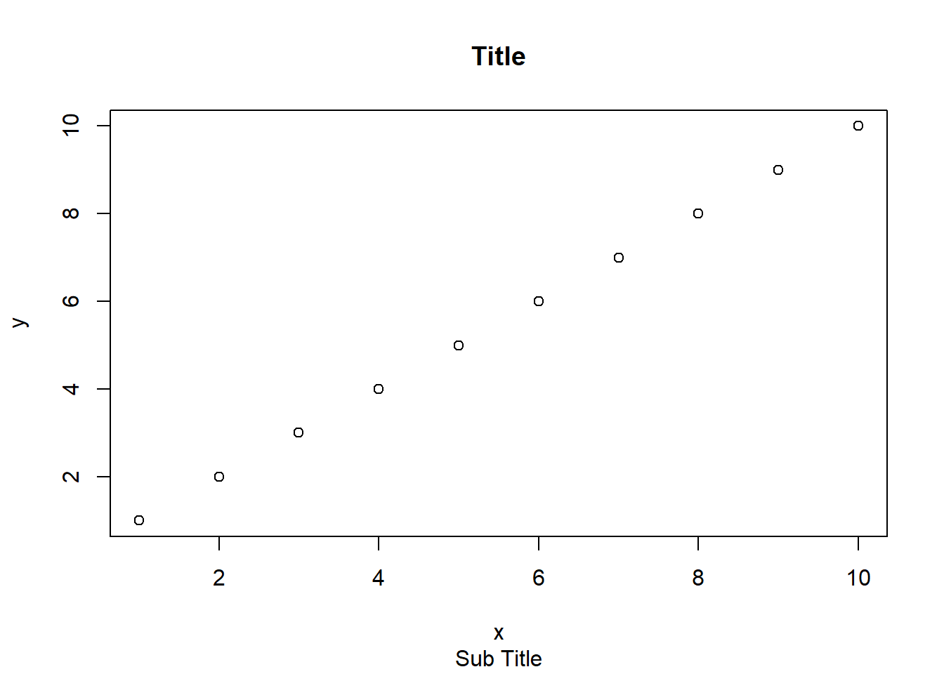
Label
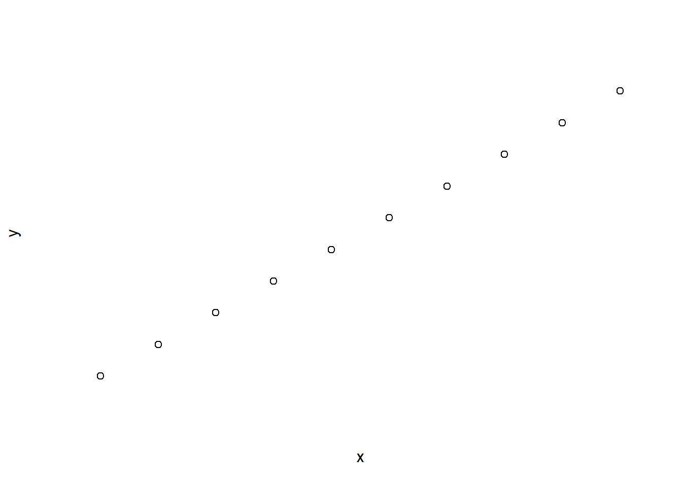
No title and label
ann annotation
It is nearly the same as xlab = "" and ylab = "".
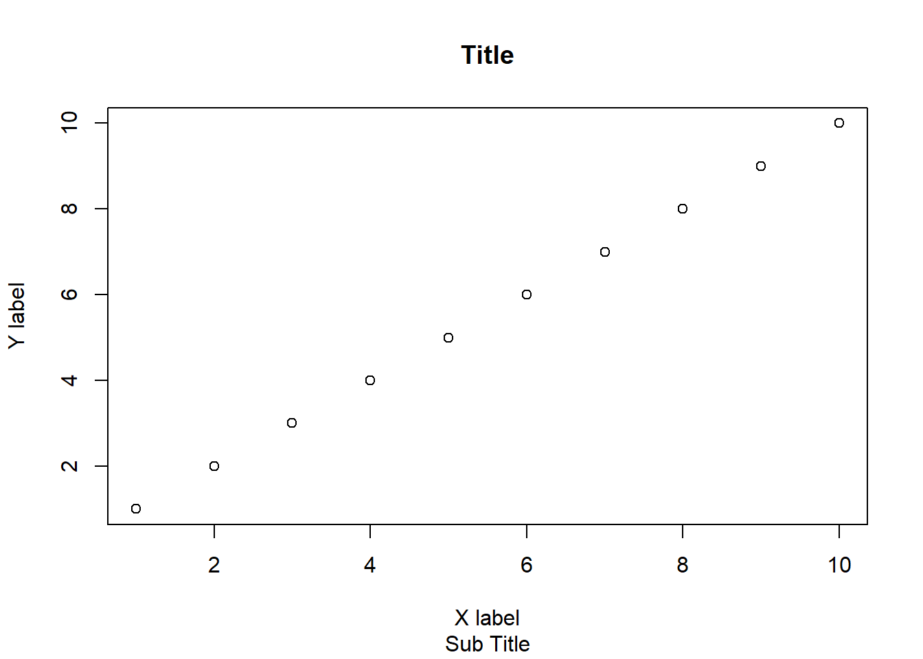
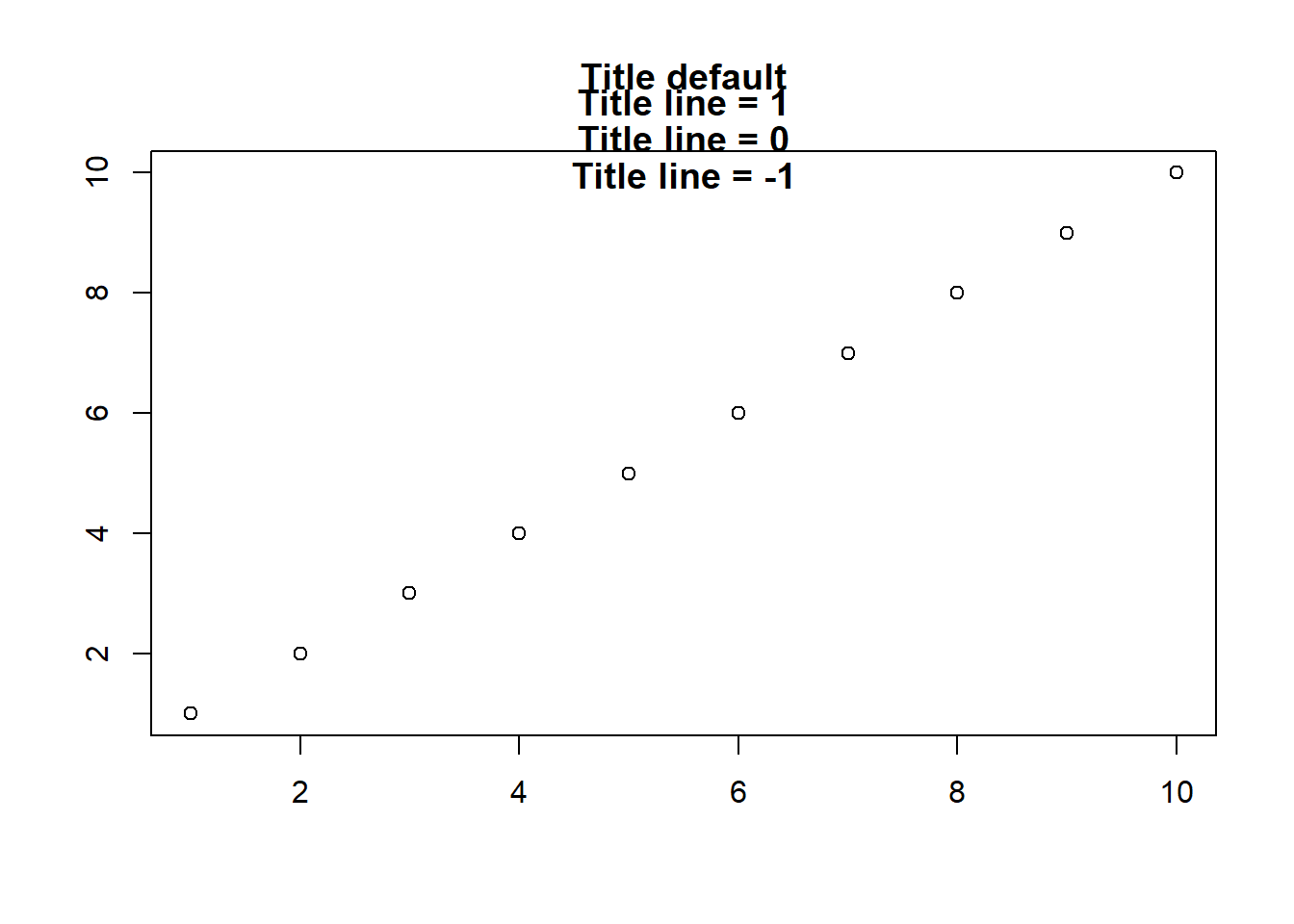
Add title and labels
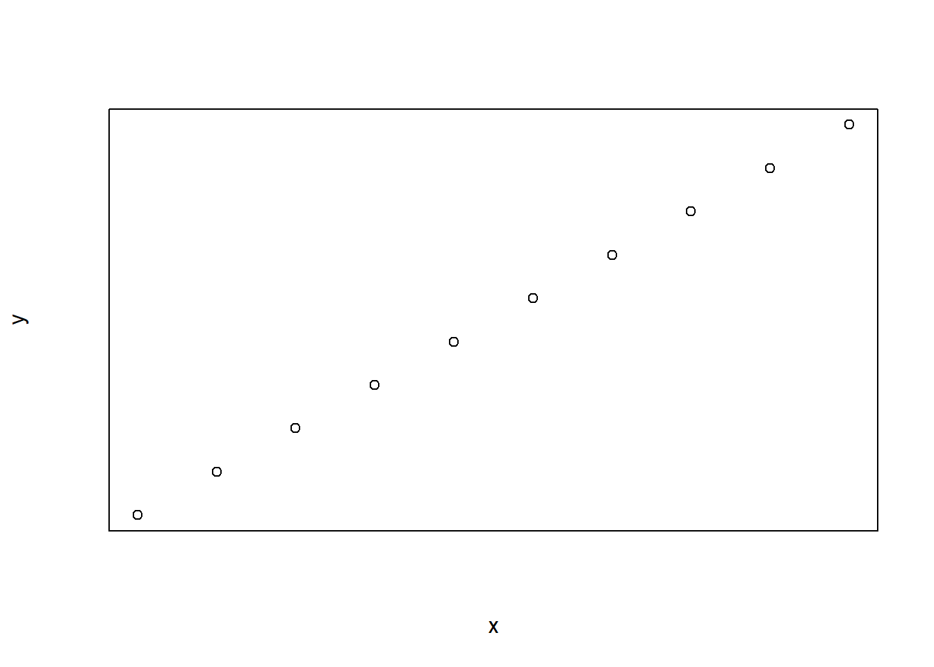
Axis
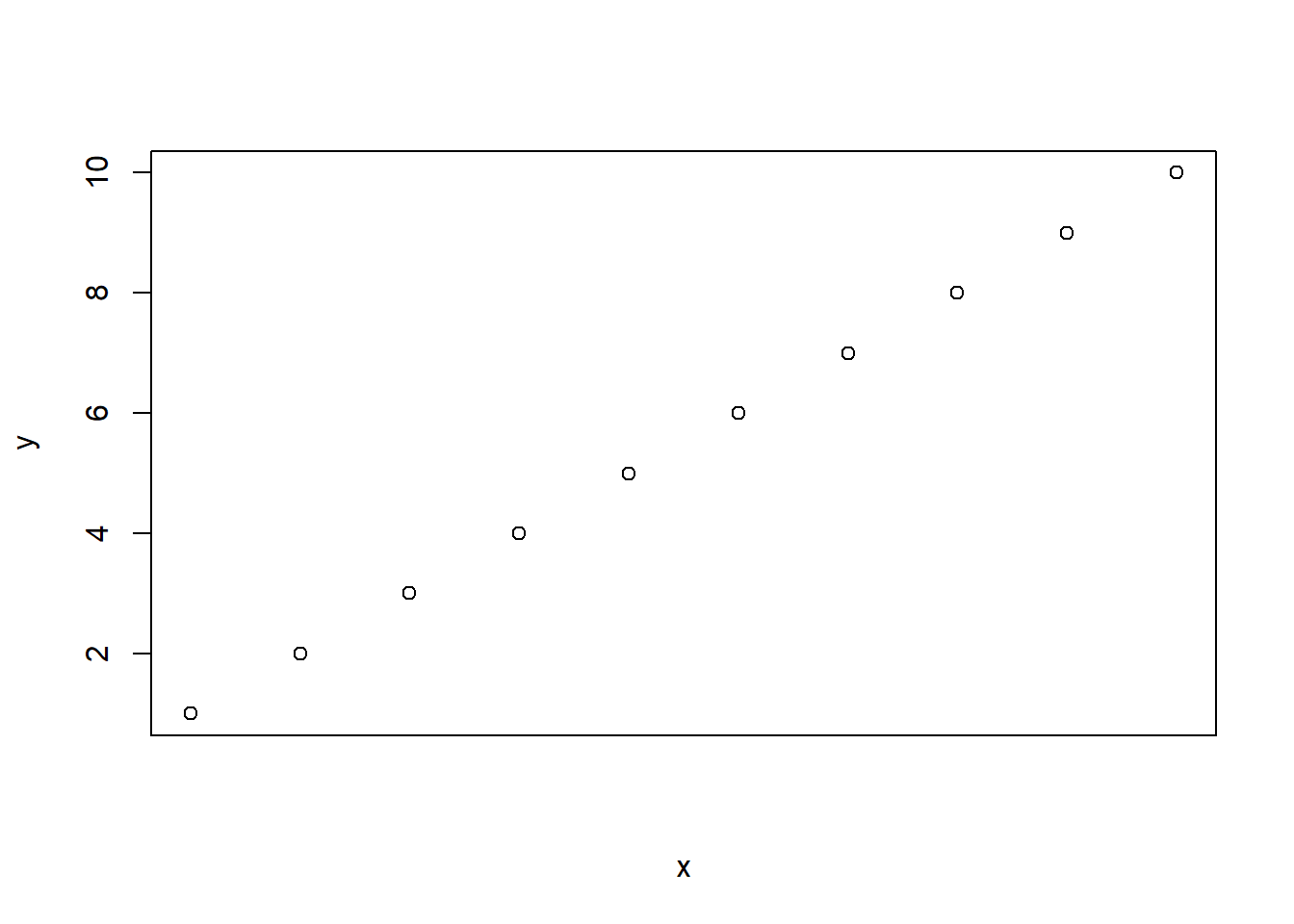
Axis tick
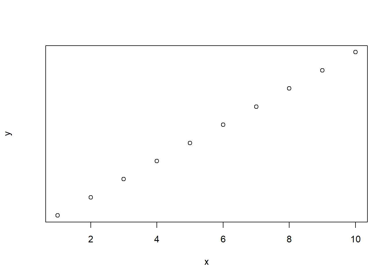
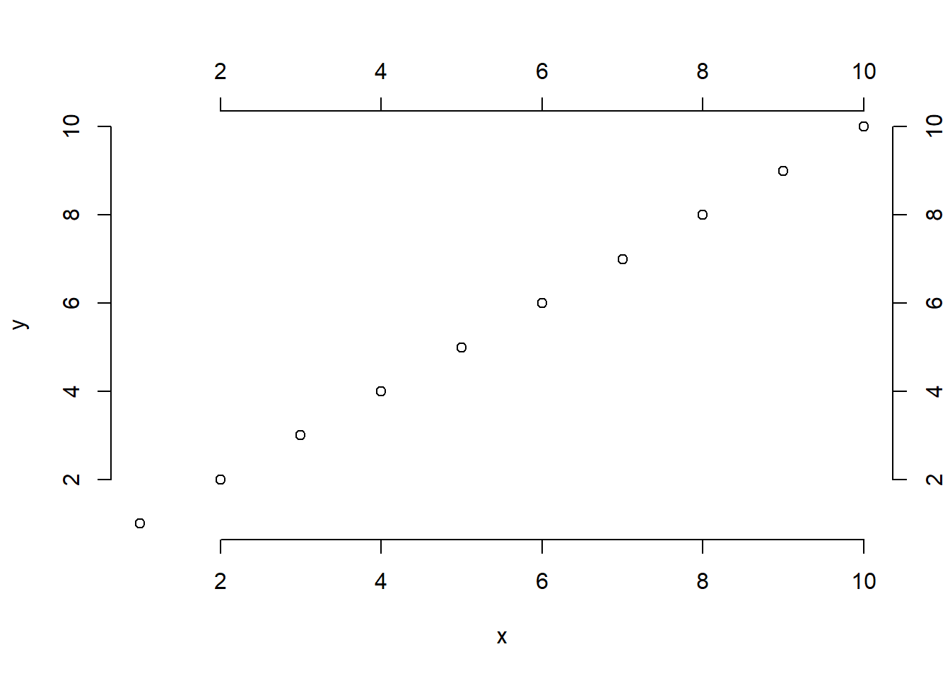
Read more
Plot symbol
-
NA: No symbol -
0:25: Defined symbols
x <- rep(1:5, 5)
y <- rep(5:1, each = 5)
plot(x, y, pch = 1:25, cex = 2, ylim = c(1, 6), axes = FALSE, xlab = "", ylab = "", col = 2, bg = 3)
text(x, y+0.3, 1:25)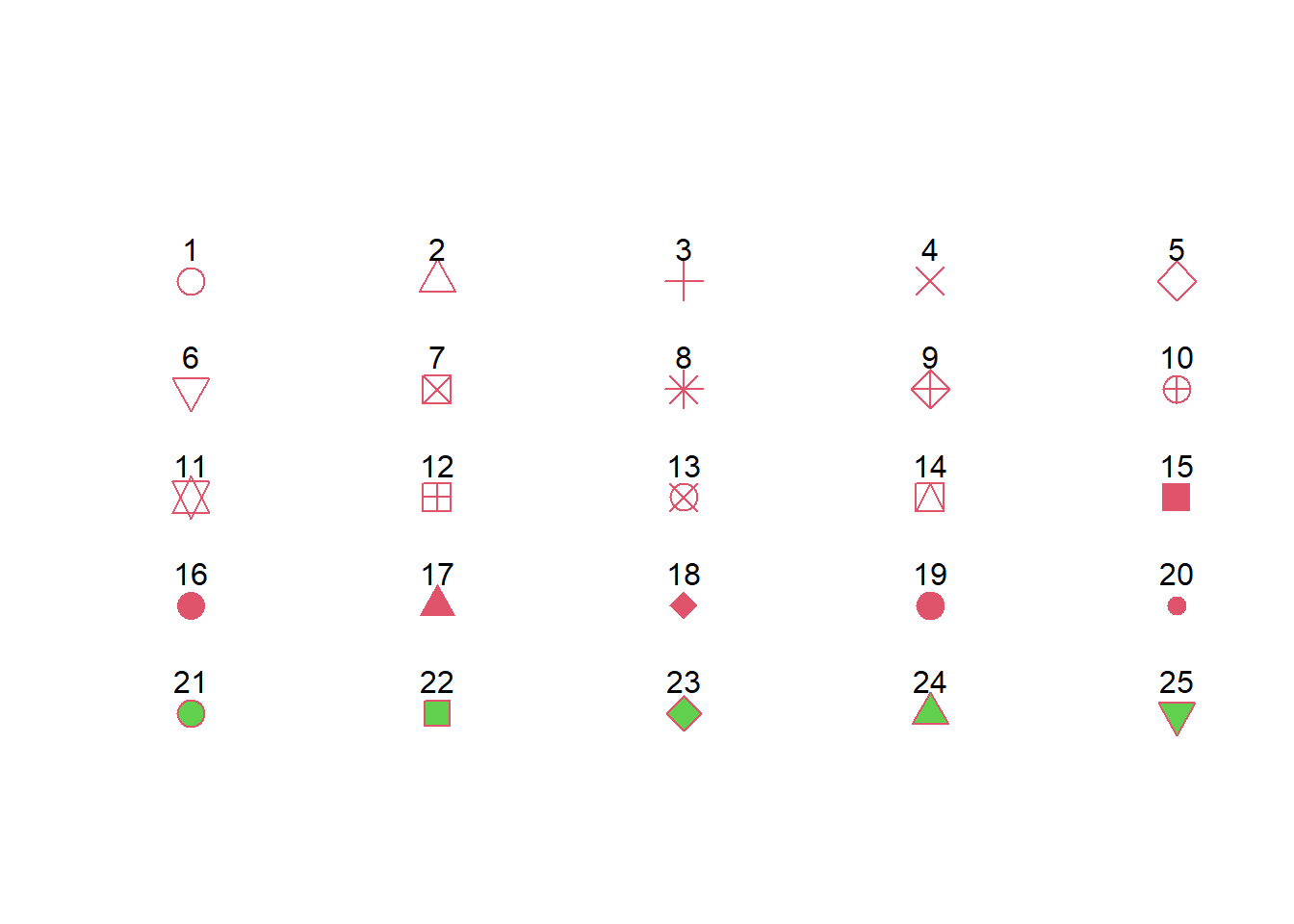
21:25 can have different border and fill colors. In this example, The border color is red (col = 2) and the fill color is green (bg = 3), respectively.
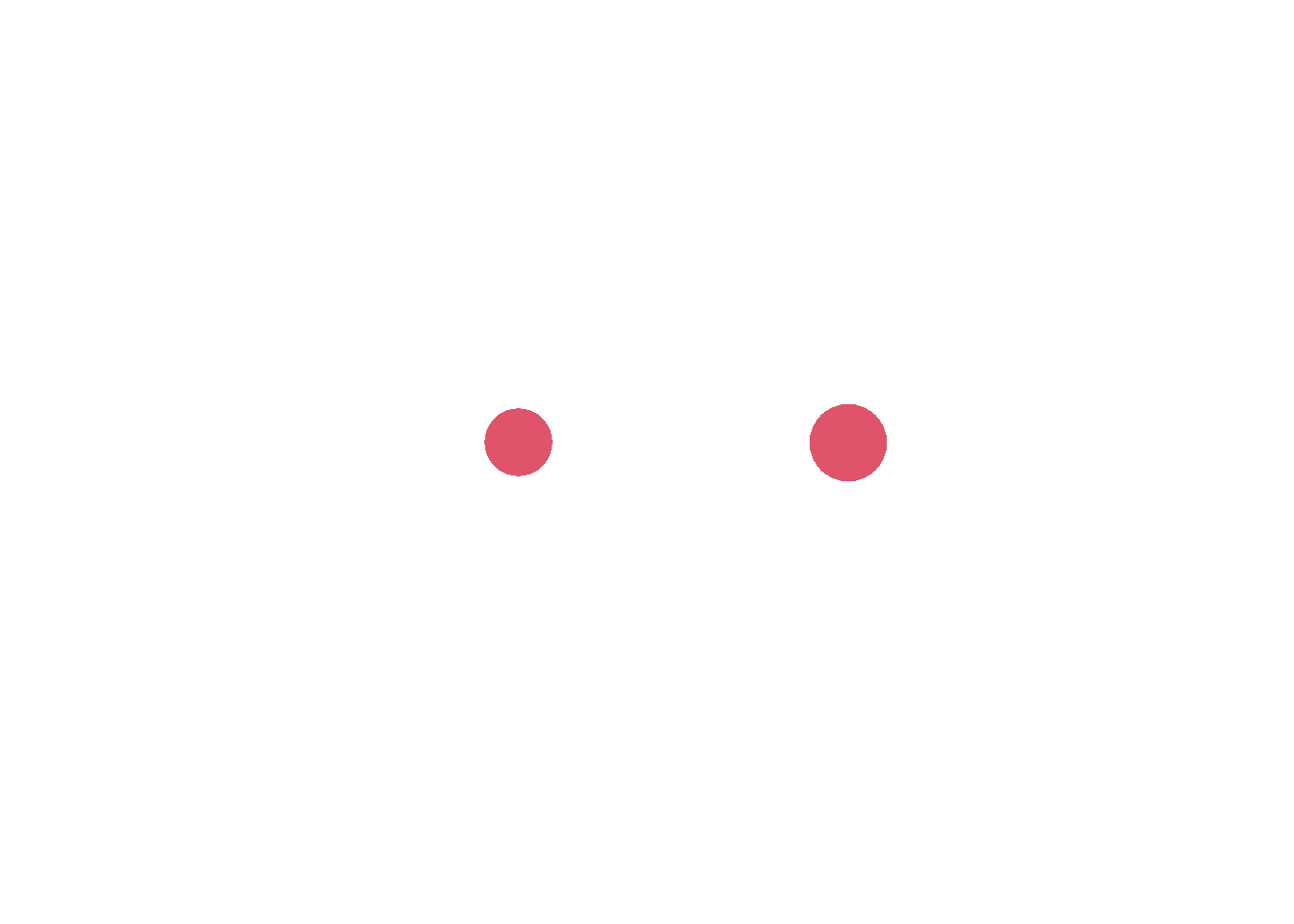
Differences among 16, 19, 20, and 21
-
pch = 16: simple solid circle -
pch = 19: solid circle which have border -
pch = 20: solid circle which size is 2/3 ofpch = 19 -
pch = 21: filled circle which can have different border and fill colors.
Especially, the difference between pch = 16 and pch = 19 is subtle. pch = 19 has border. When lwd is applied, it has bigger size than pch = 16 by the boundary line.
pch = 26:31
pch = 26:31 are unued.
This show warning messages like below.
Warning messages:
1: In plot.xy(xy, type, ...) : unimplemented pch value '26'
2: In plot.xy(xy, type, ...) : unimplemented pch value '27'
3: In plot.xy(xy, type, ...) : unimplemented pch value '28'
4: In plot.xy(xy, type, ...) : unimplemented pch value '29'
5: In plot.xy(xy, type, ...) : unimplemented pch value '30'
6: In plot.xy(xy, type, ...) : unimplemented pch value '31'
pch = 32:127
pch = 32:127 are correspond to ASCII characters. You can see these characters Here.
x <- rep(1:10)
y <- rep(1, 10)
plot(x, y, pch = 33:42, cex = 2, axes = FALSE, xlab = "", ylab = "")
text(x, y+0.1, 33:42)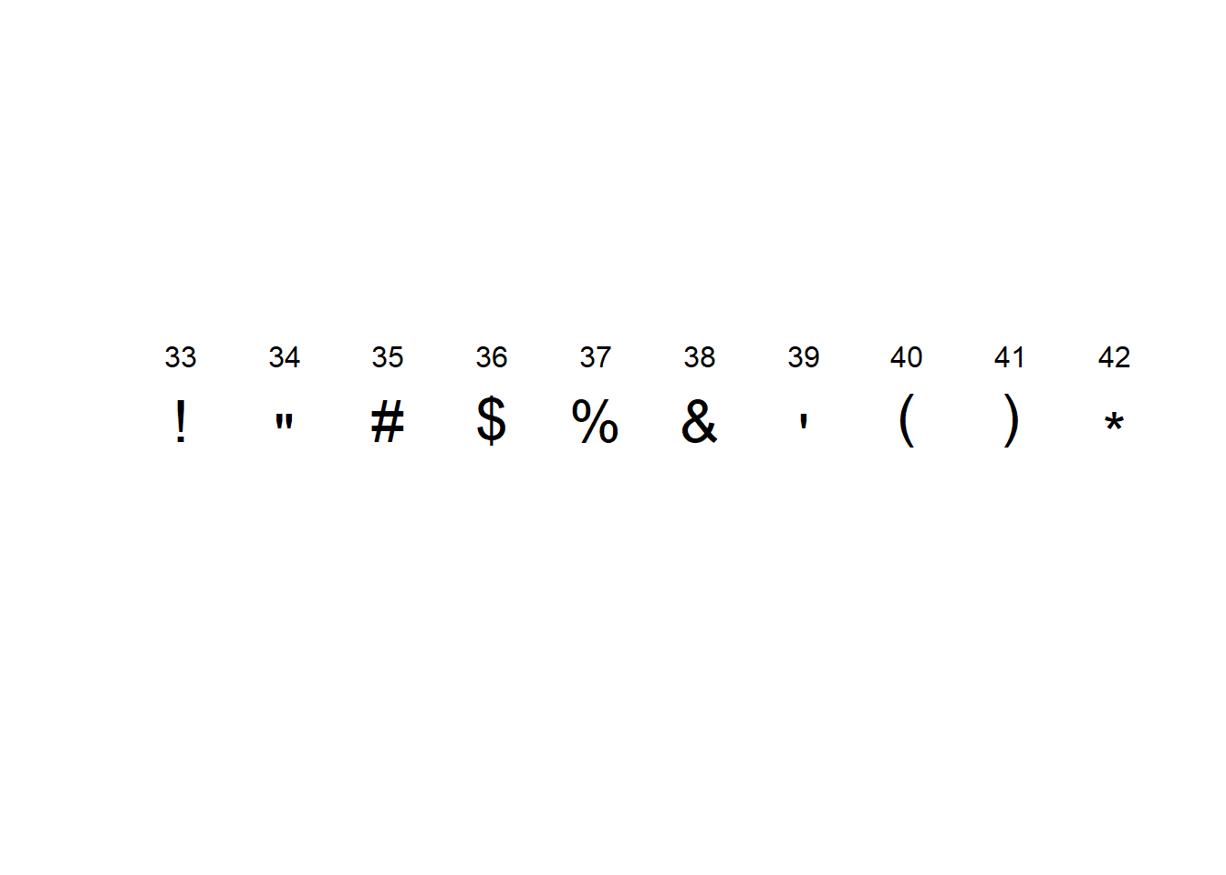
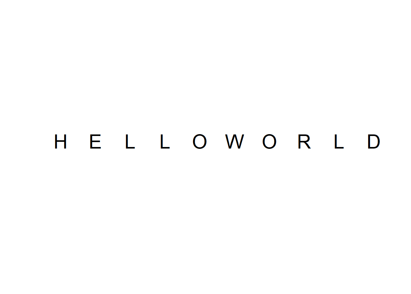
You can also specify characters directly.
Read more
pch plotting character ?pch show details
Plot type
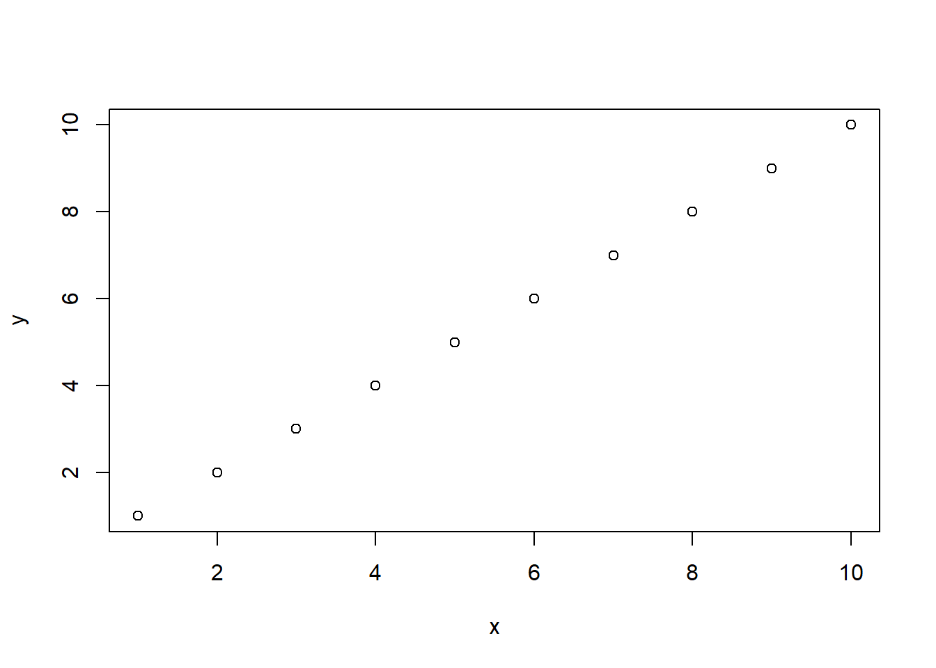
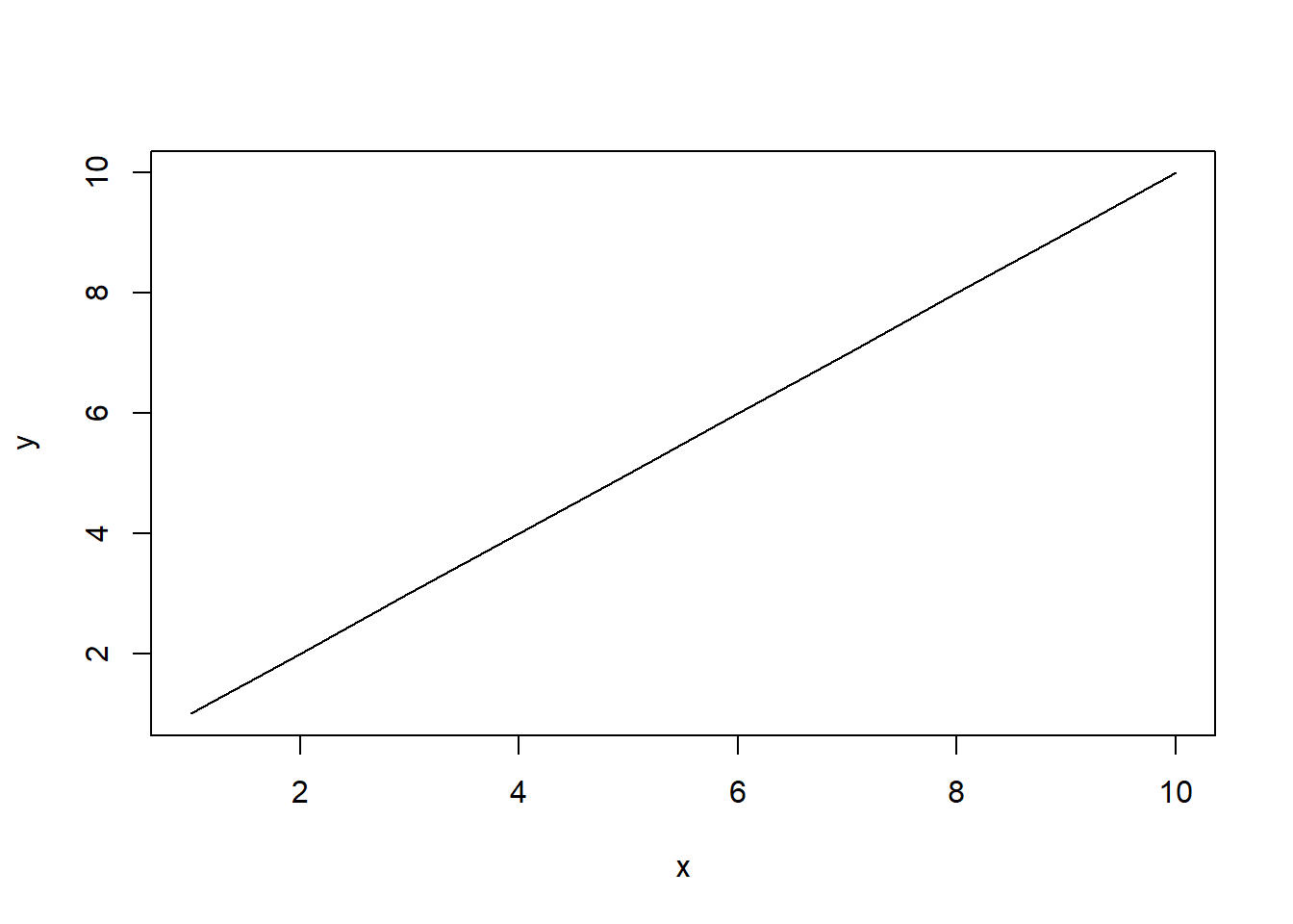
The type of plot is specified by the type argument to plot().
- “
p”: points - “
l”: lines - “
c”: empty points joined by lines - “
o”: overplotted points and lines - “
s” and “S”: stair steps - “
h”: histogram-like vertical lines - “
n”: no point or line
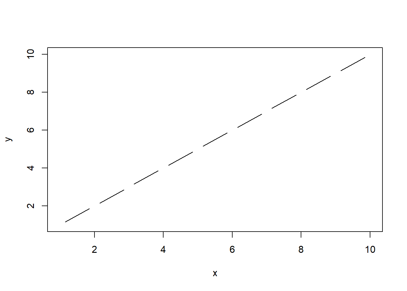
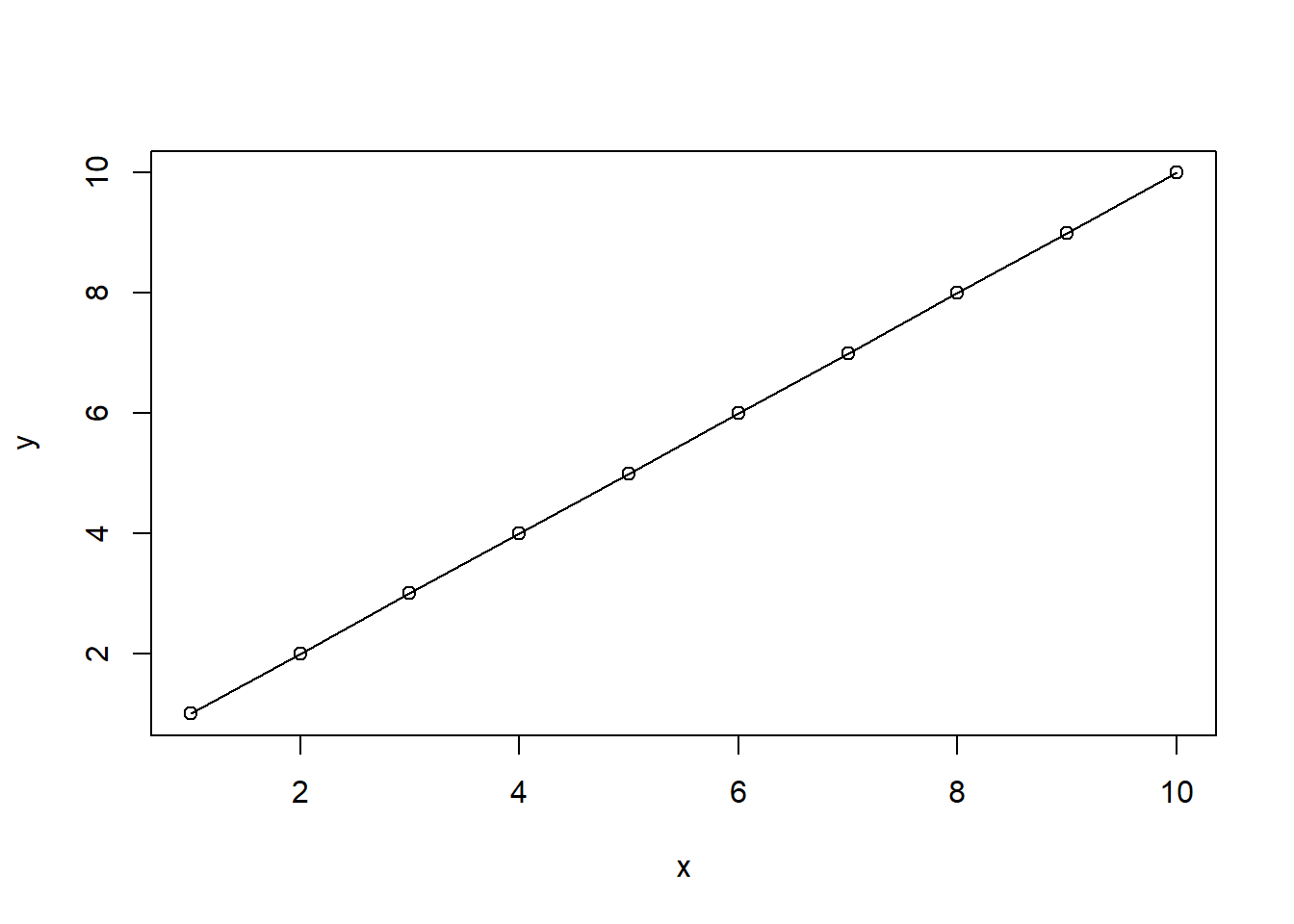
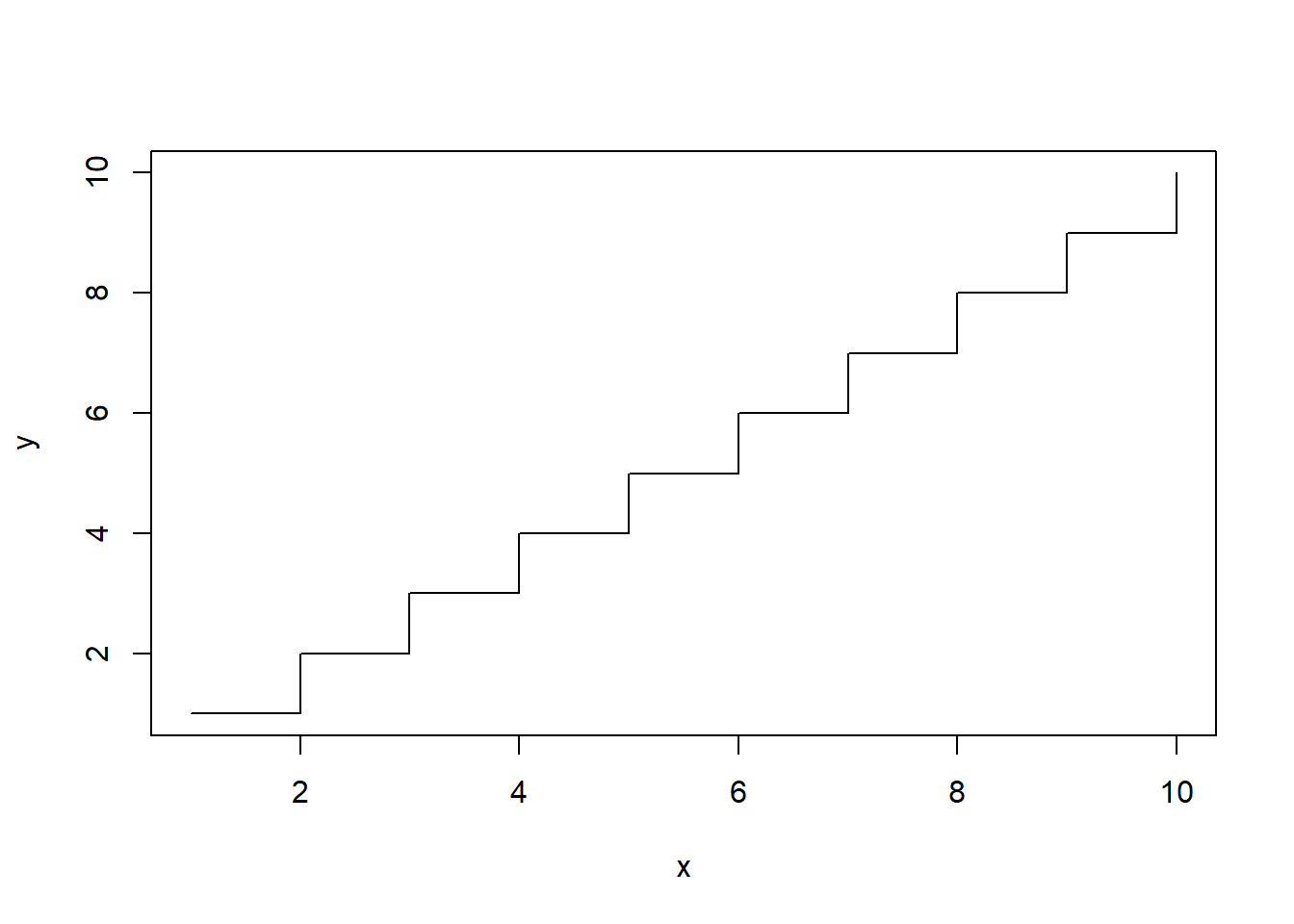
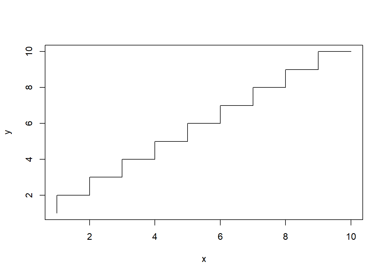
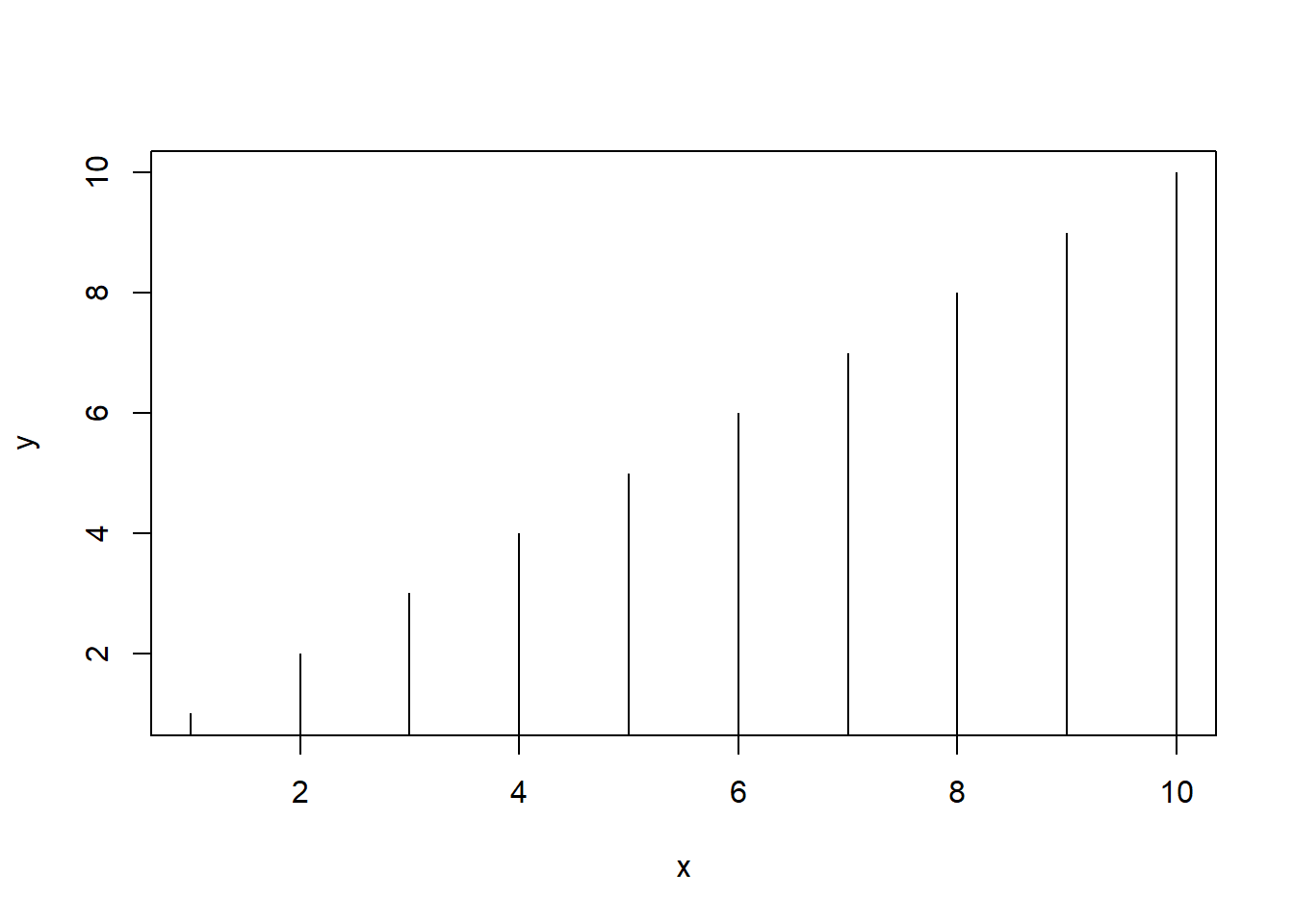
type = "n" is used for overwriting plots or lines.
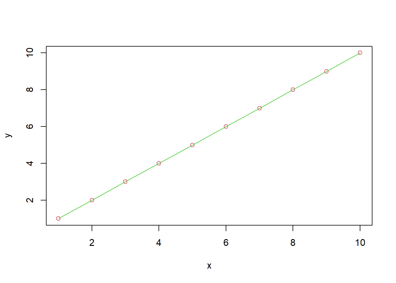
When overwriting, please pay attention xlim and ylim. If the points or lines to be drawn later does not fit on the range of first canvas plot, they will not appear.
Character or symbol size
character expansion(cex)
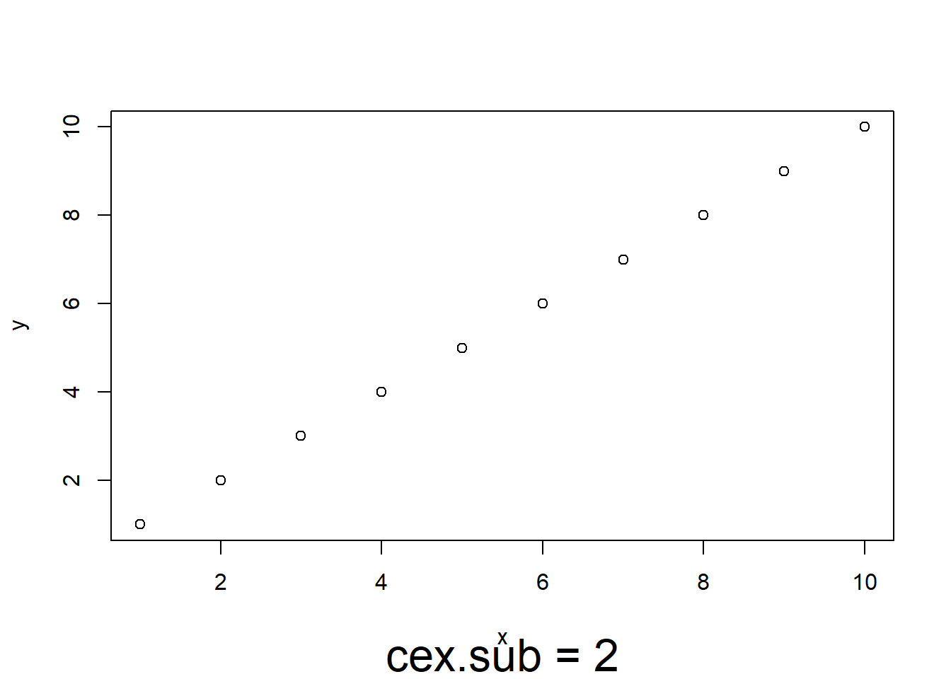
cex.axiscex.labcex.maincex.sub
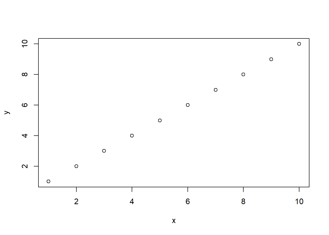
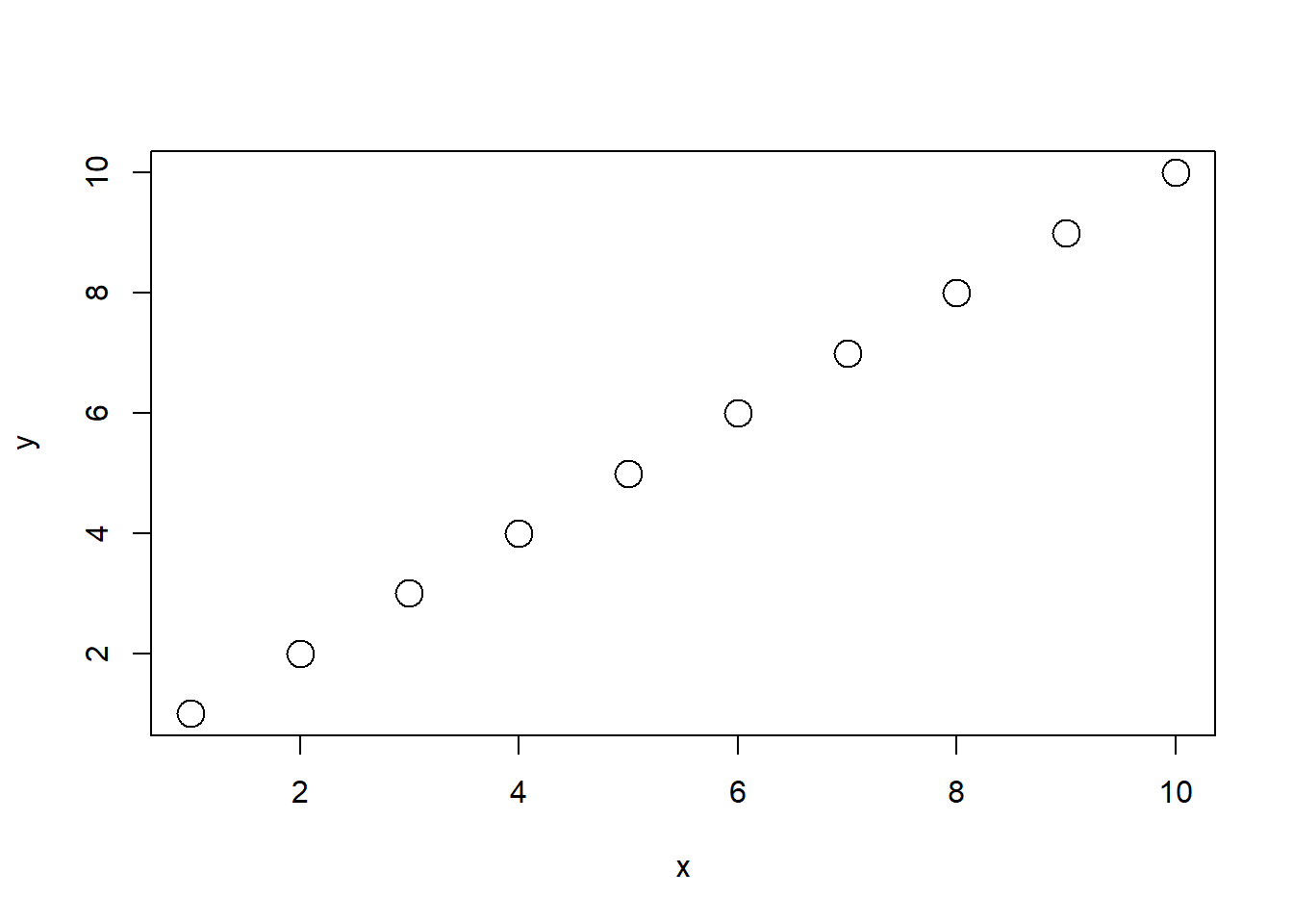
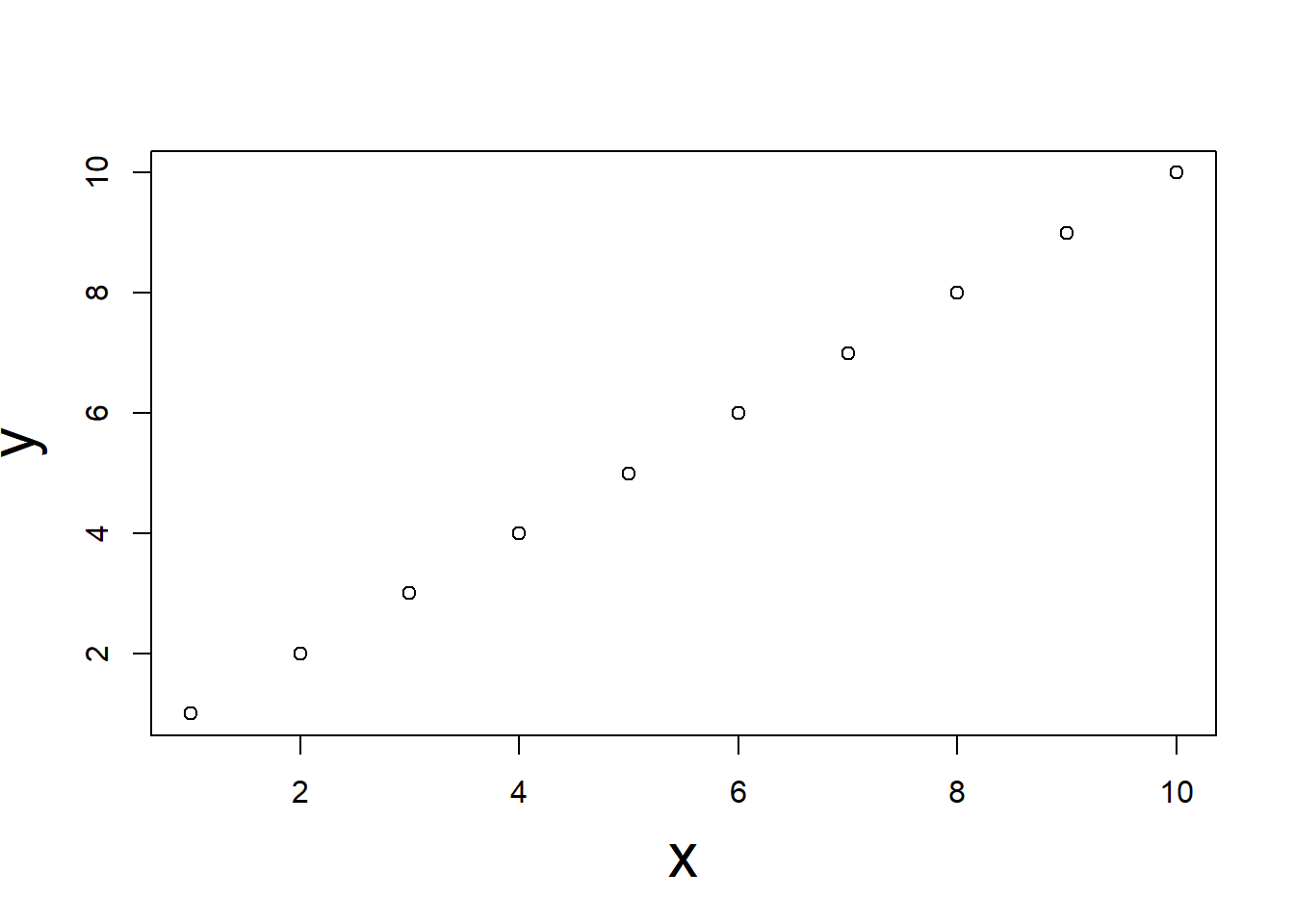
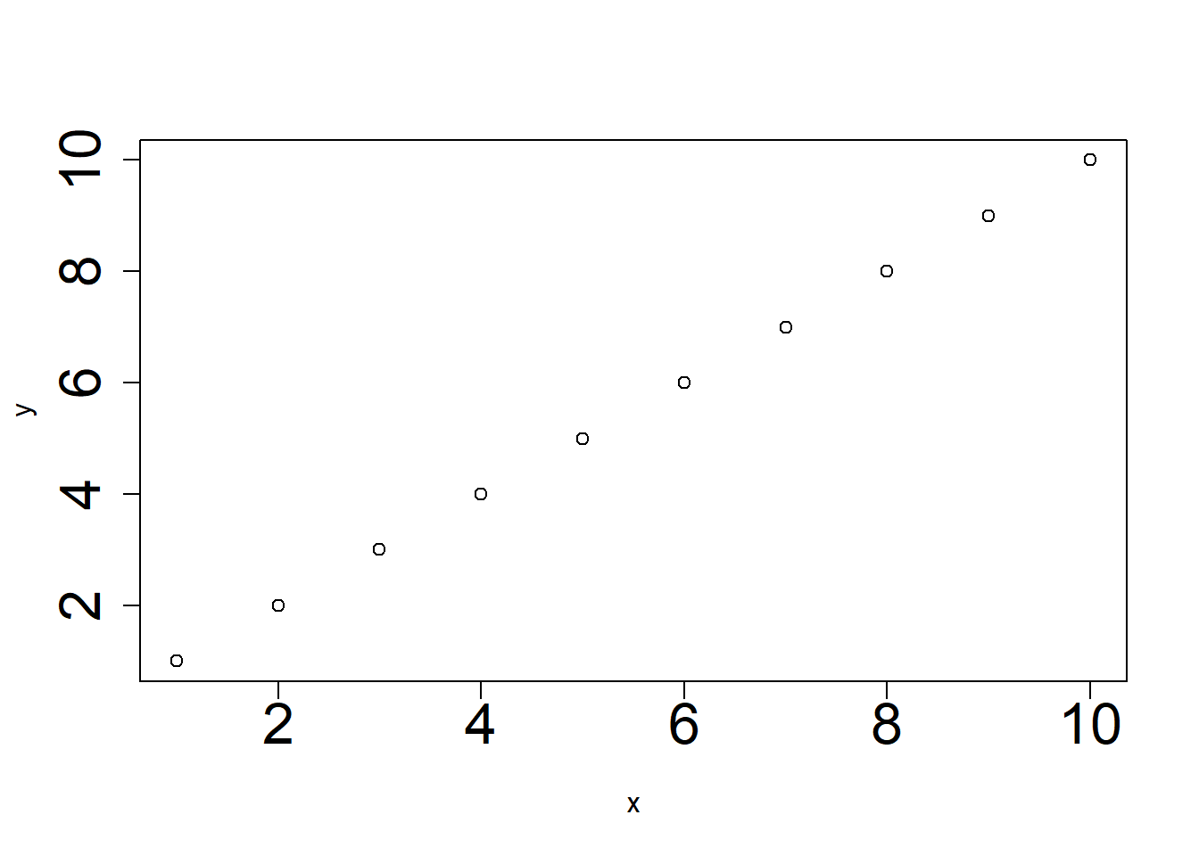
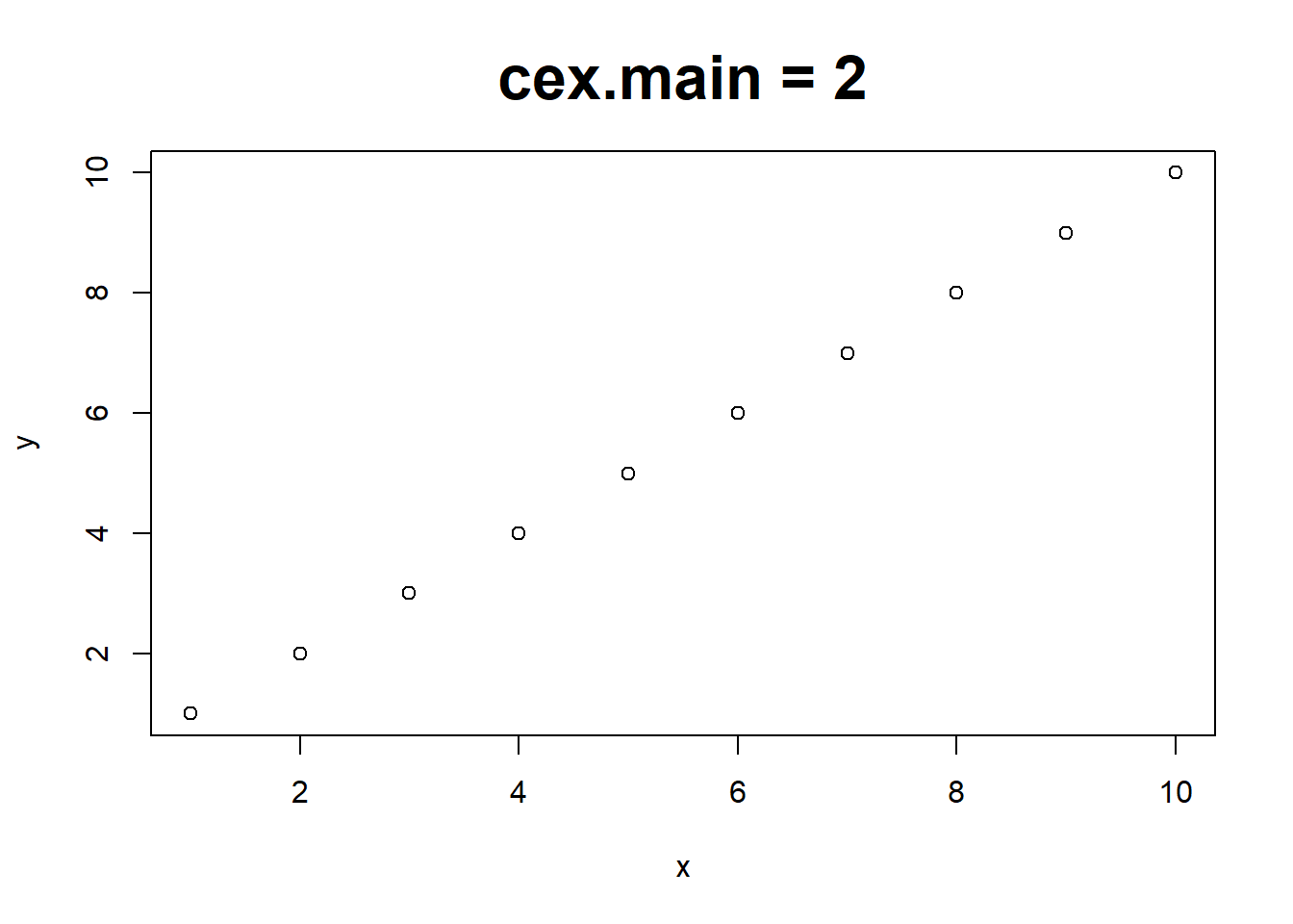
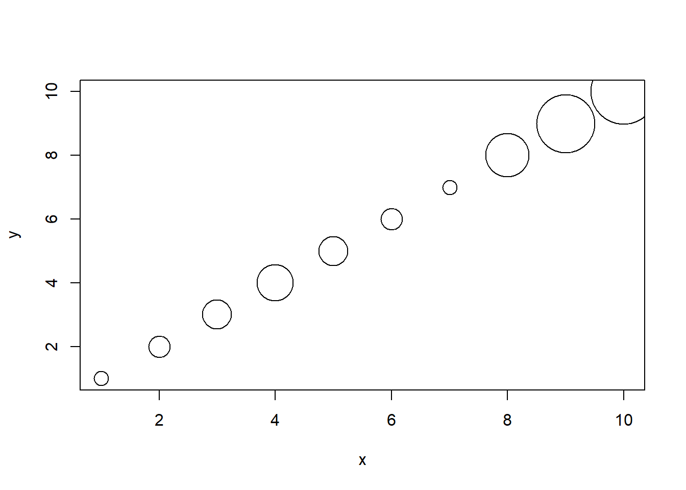
cex can apply each points. The point size can be changed according to the point values. This can be used to create a bubble chart.
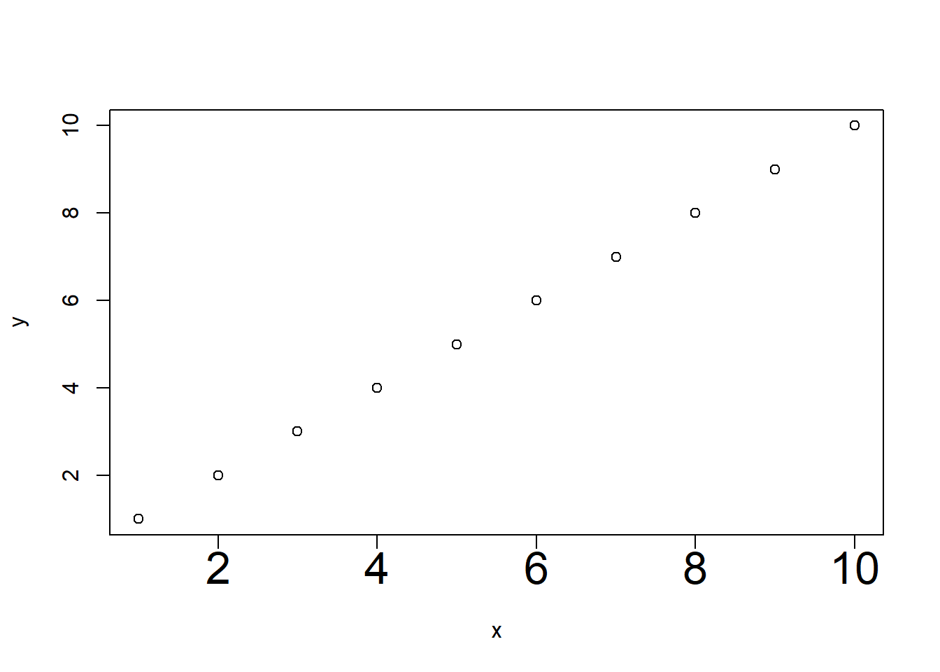
If you want to magnify only x or y label(axis), you can draw it later and specify cex for it.
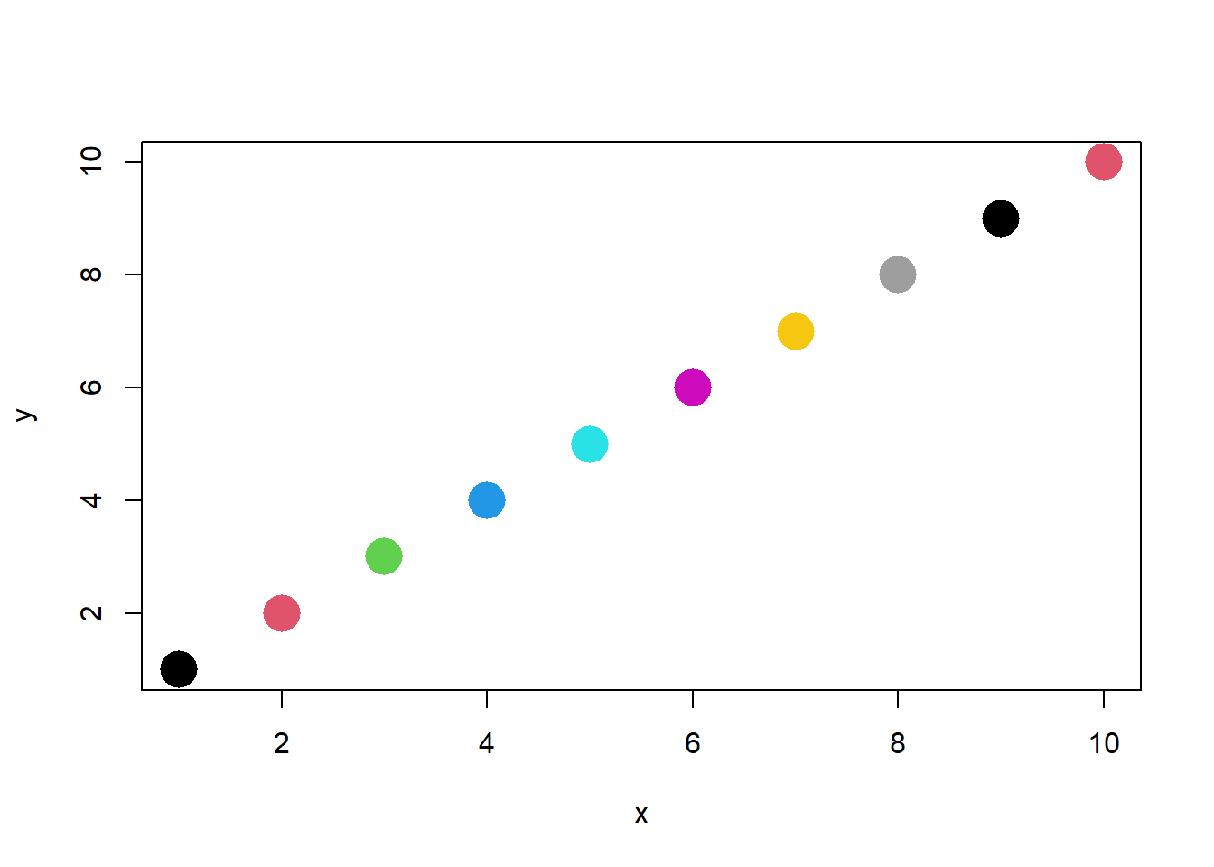
Color
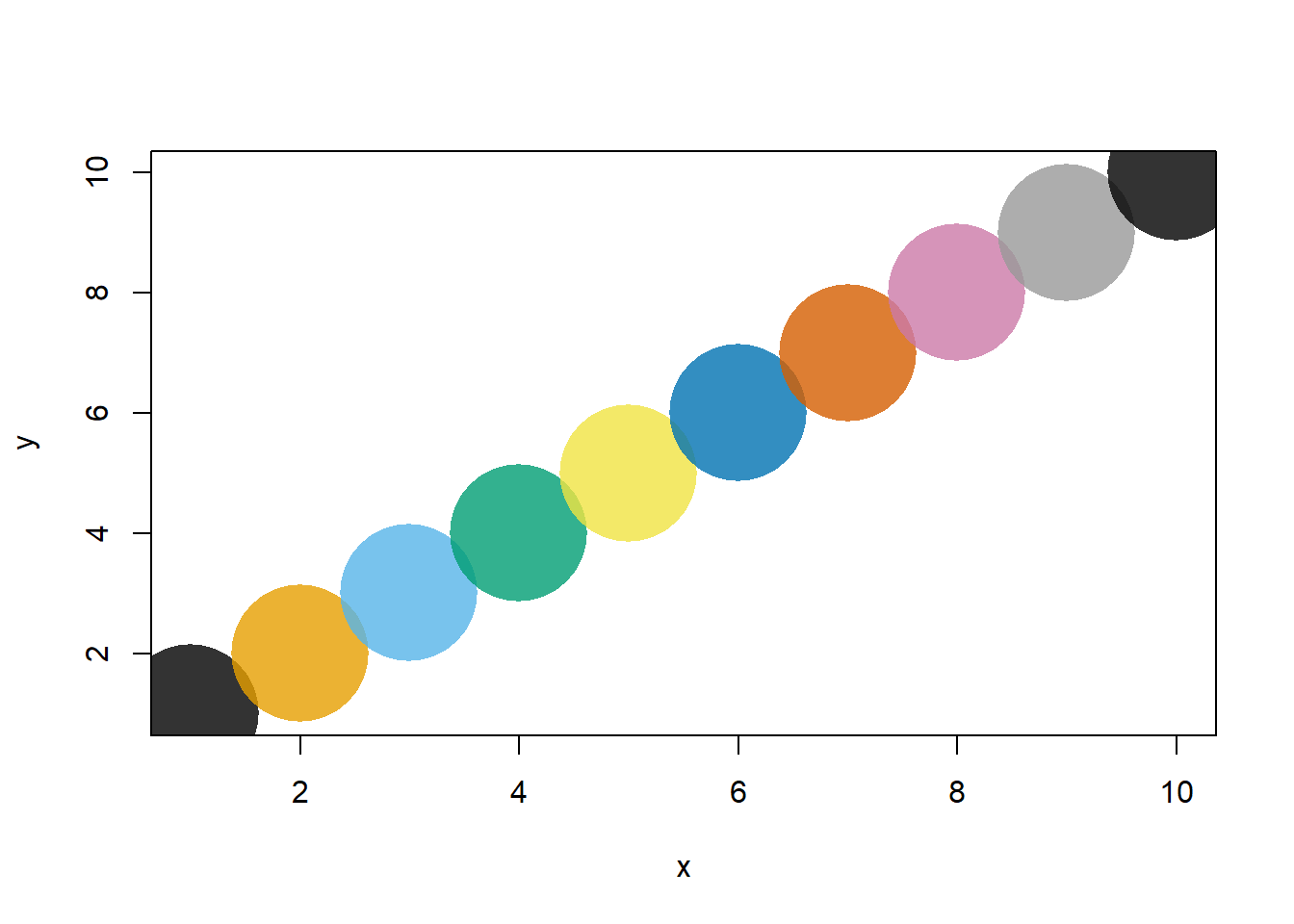
 [1] "R3"              "R4"              "ggplot2"         "Okabe-Ito"
 [5] "Accent"          "Dark 2"          "Paired"          "Pastel 1"
 [9] "Pastel 2"        "Set 1"           "Set 2"           "Set 3"
[13] "Tableau 10" "Classic Tableau" "Polychrome 36" "Alphabet" [1] "black" "#E69F00" "#56B4E9" "#009E73" "#F0E442" "#0072B2" "#D55E00"
[8] "#CC79A7" "gray60" [1] "#000000" "#E69F00" "#56B4E9" "#009E73" "#F0E442" "#0072B2" "#D55E00"
[8] "#CC79A7" "#999999"Transparency
Defined color name
[1] "white" "aliceblue" "antiquewhite"
[4] "antiquewhite1" "antiquewhite2" "antiquewhite3"
[7] "antiquewhite4" "aquamarine" "aquamarine1"
[10] "aquamarine2" "aquamarine3" "aquamarine4"
[13] "azure" "azure1" "azure2"
[16] "azure3" "azure4" "beige"
[19] "bisque" "bisque1" "bisque2"
[22] "bisque3" "bisque4" "black"
[25] "blanchedalmond" "blue" "blue1"
[28] "blue2" "blue3" "blue4"
[31] "blueviolet" "brown" "brown1"
[34] "brown2" "brown3" "brown4"
[37] "burlywood" "burlywood1" "burlywood2"
[40] "burlywood3" "burlywood4" "cadetblue"
[43] "cadetblue1" "cadetblue2" "cadetblue3"
[46] "cadetblue4" "chartreuse" "chartreuse1"
[49] "chartreuse2" "chartreuse3" "chartreuse4"
[52] "chocolate" "chocolate1" "chocolate2"
[55] "chocolate3" "chocolate4" "coral"
[58] "coral1" "coral2" "coral3"
[61] "coral4" "cornflowerblue" "cornsilk"
[64] "cornsilk1" "cornsilk2" "cornsilk3"
[67] "cornsilk4" "cyan" "cyan1"
[70] "cyan2" "cyan3" "cyan4"
[73] "darkblue" "darkcyan" "darkgoldenrod"
[76] "darkgoldenrod1" "darkgoldenrod2" "darkgoldenrod3"
[79] "darkgoldenrod4" "darkgray" "darkgreen"
[82] "darkgrey" "darkkhaki" "darkmagenta"
[85] "darkolivegreen" "darkolivegreen1" "darkolivegreen2"
[88] "darkolivegreen3" "darkolivegreen4" "darkorange"
[91] "darkorange1" "darkorange2" "darkorange3"
[94] "darkorange4" "darkorchid" "darkorchid1"
[97] "darkorchid2" "darkorchid3" "darkorchid4"
[100] "darkred" "darksalmon" "darkseagreen"
[103] "darkseagreen1" "darkseagreen2" "darkseagreen3"
[106] "darkseagreen4" "darkslateblue" "darkslategray"
[109] "darkslategray1" "darkslategray2" "darkslategray3"
[112] "darkslategray4" "darkslategrey" "darkturquoise"
[115] "darkviolet" "deeppink" "deeppink1"
[118] "deeppink2" "deeppink3" "deeppink4"
[121] "deepskyblue" "deepskyblue1" "deepskyblue2"
[124] "deepskyblue3" "deepskyblue4" "dimgray"
[127] "dimgrey" "dodgerblue" "dodgerblue1"
[130] "dodgerblue2" "dodgerblue3" "dodgerblue4"
[133] "firebrick" "firebrick1" "firebrick2"
[136] "firebrick3" "firebrick4" "floralwhite"
[139] "forestgreen" "gainsboro" "ghostwhite"
[142] "gold" "gold1" "gold2"
[145] "gold3" "gold4" "goldenrod"
[148] "goldenrod1" "goldenrod2" "goldenrod3"
[151] "goldenrod4" "gray" "gray0"
[154] "gray1" "gray2" "gray3"
[157] "gray4" "gray5" "gray6"
[160] "gray7" "gray8" "gray9"
[163] "gray10" "gray11" "gray12"
[166] "gray13" "gray14" "gray15"
[169] "gray16" "gray17" "gray18"
[172] "gray19" "gray20" "gray21"
[175] "gray22" "gray23" "gray24"
[178] "gray25" "gray26" "gray27"
[181] "gray28" "gray29" "gray30"
[184] "gray31" "gray32" "gray33"
[187] "gray34" "gray35" "gray36"
[190] "gray37" "gray38" "gray39"
[193] "gray40" "gray41" "gray42"
[196] "gray43" "gray44" "gray45"
[199] "gray46" "gray47" "gray48"
[202] "gray49" "gray50" "gray51"
[205] "gray52" "gray53" "gray54"
[208] "gray55" "gray56" "gray57"
[211] "gray58" "gray59" "gray60"
[214] "gray61" "gray62" "gray63"
[217] "gray64" "gray65" "gray66"
[220] "gray67" "gray68" "gray69"
[223] "gray70" "gray71" "gray72"
[226] "gray73" "gray74" "gray75"
[229] "gray76" "gray77" "gray78"
[232] "gray79" "gray80" "gray81"
[235] "gray82" "gray83" "gray84"
[238] "gray85" "gray86" "gray87"
[241] "gray88" "gray89" "gray90"
[244] "gray91" "gray92" "gray93"
[247] "gray94" "gray95" "gray96"
[250] "gray97" "gray98" "gray99"
[253] "gray100" "green" "green1"
[256] "green2" "green3" "green4"
[259] "greenyellow" "grey" "grey0"
[262] "grey1" "grey2" "grey3"
[265] "grey4" "grey5" "grey6"
[268] "grey7" "grey8" "grey9"
[271] "grey10" "grey11" "grey12"
[274] "grey13" "grey14" "grey15"
[277] "grey16" "grey17" "grey18"
[280] "grey19" "grey20" "grey21"
[283] "grey22" "grey23" "grey24"
[286] "grey25" "grey26" "grey27"
[289] "grey28" "grey29" "grey30"
[292] "grey31" "grey32" "grey33"
[295] "grey34" "grey35" "grey36"
[298] "grey37" "grey38" "grey39"
[301] "grey40" "grey41" "grey42"
[304] "grey43" "grey44" "grey45"
[307] "grey46" "grey47" "grey48"
[310] "grey49" "grey50" "grey51"
[313] "grey52" "grey53" "grey54"
[316] "grey55" "grey56" "grey57"
[319] "grey58" "grey59" "grey60"
[322] "grey61" "grey62" "grey63"
[325] "grey64" "grey65" "grey66"
[328] "grey67" "grey68" "grey69"
[331] "grey70" "grey71" "grey72"
[334] "grey73" "grey74" "grey75"
[337] "grey76" "grey77" "grey78"
[340] "grey79" "grey80" "grey81"
[343] "grey82" "grey83" "grey84"
[346] "grey85" "grey86" "grey87"
[349] "grey88" "grey89" "grey90"
[352] "grey91" "grey92" "grey93"
[355] "grey94" "grey95" "grey96"
[358] "grey97" "grey98" "grey99"
[361] "grey100" "honeydew" "honeydew1"
[364] "honeydew2" "honeydew3" "honeydew4"
[367] "hotpink" "hotpink1" "hotpink2"
[370] "hotpink3" "hotpink4" "indianred"
[373] "indianred1" "indianred2" "indianred3"
[376] "indianred4" "ivory" "ivory1"
[379] "ivory2" "ivory3" "ivory4"
[382] "khaki" "khaki1" "khaki2"
[385] "khaki3" "khaki4" "lavender"
[388] "lavenderblush" "lavenderblush1" "lavenderblush2"
[391] "lavenderblush3" "lavenderblush4" "lawngreen"
[394] "lemonchiffon" "lemonchiffon1" "lemonchiffon2"
[397] "lemonchiffon3" "lemonchiffon4" "lightblue"
[400] "lightblue1" "lightblue2" "lightblue3"
[403] "lightblue4" "lightcoral" "lightcyan"
[406] "lightcyan1" "lightcyan2" "lightcyan3"
[409] "lightcyan4" "lightgoldenrod" "lightgoldenrod1"
[412] "lightgoldenrod2" "lightgoldenrod3" "lightgoldenrod4"
[415] "lightgoldenrodyellow" "lightgray" "lightgreen"
[418] "lightgrey" "lightpink" "lightpink1"
[421] "lightpink2" "lightpink3" "lightpink4"
[424] "lightsalmon" "lightsalmon1" "lightsalmon2"
[427] "lightsalmon3" "lightsalmon4" "lightseagreen"
[430] "lightskyblue" "lightskyblue1" "lightskyblue2"
[433] "lightskyblue3" "lightskyblue4" "lightslateblue"
[436] "lightslategray" "lightslategrey" "lightsteelblue"
[439] "lightsteelblue1" "lightsteelblue2" "lightsteelblue3"
[442] "lightsteelblue4" "lightyellow" "lightyellow1"
[445] "lightyellow2" "lightyellow3" "lightyellow4"
[448] "limegreen" "linen" "magenta"
[451] "magenta1" "magenta2" "magenta3"
[454] "magenta4" "maroon" "maroon1"
[457] "maroon2" "maroon3" "maroon4"
[460] "mediumaquamarine" "mediumblue" "mediumorchid"
[463] "mediumorchid1" "mediumorchid2" "mediumorchid3"
[466] "mediumorchid4" "mediumpurple" "mediumpurple1"
[469] "mediumpurple2" "mediumpurple3" "mediumpurple4"
[472] "mediumseagreen" "mediumslateblue" "mediumspringgreen"
[475] "mediumturquoise" "mediumvioletred" "midnightblue"
[478] "mintcream" "mistyrose" "mistyrose1"
[481] "mistyrose2" "mistyrose3" "mistyrose4"
[484] "moccasin" "navajowhite" "navajowhite1"
[487] "navajowhite2" "navajowhite3" "navajowhite4"
[490] "navy" "navyblue" "oldlace"
[493] "olivedrab" "olivedrab1" "olivedrab2"
[496] "olivedrab3" "olivedrab4" "orange"
[499] "orange1" "orange2" "orange3"
[502] "orange4" "orangered" "orangered1"
[505] "orangered2" "orangered3" "orangered4"
[508] "orchid" "orchid1" "orchid2"
[511] "orchid3" "orchid4" "palegoldenrod"
[514] "palegreen" "palegreen1" "palegreen2"
[517] "palegreen3" "palegreen4" "paleturquoise"
[520] "paleturquoise1" "paleturquoise2" "paleturquoise3"
[523] "paleturquoise4" "palevioletred" "palevioletred1"
[526] "palevioletred2" "palevioletred3" "palevioletred4"
[529] "papayawhip" "peachpuff" "peachpuff1"
[532] "peachpuff2" "peachpuff3" "peachpuff4"
[535] "peru" "pink" "pink1"
[538] "pink2" "pink3" "pink4"
[541] "plum" "plum1" "plum2"
[544] "plum3" "plum4" "powderblue"
[547] "purple" "purple1" "purple2"
[550] "purple3" "purple4" "red"
[553] "red1" "red2" "red3"
[556] "red4" "rosybrown" "rosybrown1"
[559] "rosybrown2" "rosybrown3" "rosybrown4"
[562] "royalblue" "royalblue1" "royalblue2"
[565] "royalblue3" "royalblue4" "saddlebrown"
[568] "salmon" "salmon1" "salmon2"
[571] "salmon3" "salmon4" "sandybrown"
[574] "seagreen" "seagreen1" "seagreen2"
[577] "seagreen3" "seagreen4" "seashell"
[580] "seashell1" "seashell2" "seashell3"
[583] "seashell4" "sienna" "sienna1"
[586] "sienna2" "sienna3" "sienna4"
[589] "skyblue" "skyblue1" "skyblue2"
[592] "skyblue3" "skyblue4" "slateblue"
[595] "slateblue1" "slateblue2" "slateblue3"
[598] "slateblue4" "slategray" "slategray1"
[601] "slategray2" "slategray3" "slategray4"
[604] "slategrey" "snow" "snow1"
[607] "snow2" "snow3" "snow4"
[610] "springgreen" "springgreen1" "springgreen2"
[613] "springgreen3" "springgreen4" "steelblue"
[616] "steelblue1" "steelblue2" "steelblue3"
[619] "steelblue4" "tan" "tan1"
[622] "tan2" "tan3" "tan4"
[625] "thistle" "thistle1" "thistle2"
[628] "thistle3" "thistle4" "tomato"
[631] "tomato1" "tomato2" "tomato3"
[634] "tomato4" "turquoise" "turquoise1"
[637] "turquoise2" "turquoise3" "turquoise4"
[640] "violet" "violetred" "violetred1"
[643] "violetred2" "violetred3" "violetred4"
[646] "wheat" "wheat1" "wheat2"
[649] "wheat3" "wheat4" "whitesmoke"
[652] "yellow" "yellow1" "yellow2"
[655] "yellow3" "yellow4" "yellowgreen"
    demo(colors)
    ---- ~~~~~~

> ### ----------- Show (almost) all named colors ---------------------
>
> ## 1) with traditional 'graphics' package:
> showCols1 <- function(bg = "gray", cex = 0.75, srt = 30) {
+     m <- ceiling(sqrt(n <- length(cl <- colors())))
+     length(cl) <- m*m; cm <- matrix(cl, m)
+     ##
+     require("graphics")
+     op <- par(mar=rep(0,4), ann=FALSE, bg = bg); on.exit(par(op))
+     plot(1:m,1:m, type="n", axes=FALSE)
+     text(col(cm), rev(row(cm)), cm,  col = cl, cex=cex, srt=srt)
+ }

> showCols1()
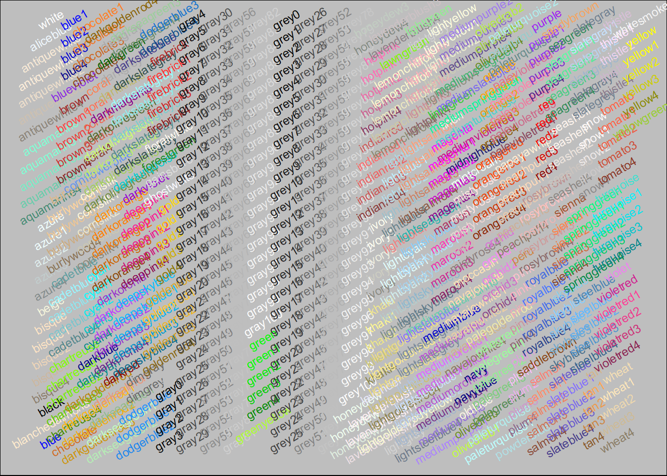
> ## 2) with 'grid' package:
> showCols2 <- function(bg = "grey", cex = 0.75, rot = 30) {
+     m <- ceiling(sqrt(n <- length(cl <- colors())))
+     length(cl) <- m*m; cm <- matrix(cl, m)
+     ##
+     require("grid")
+     grid.newpage(); vp <- viewport(width = .92, height = .92)
+     grid.rect(gp=gpar(fill=bg))
+     grid.text(cm, x = col(cm)/m, y = rev(row(cm))/m, rot = rot,
+               vp=vp, gp=gpar(cex = cex, col = cm))
+ }

> showCols2()
Loading required package: grid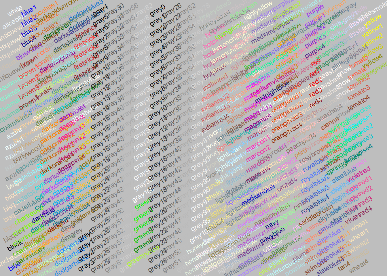
> showCols2(bg = "gray33")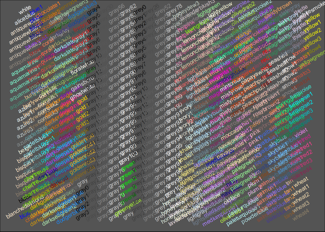
> ###
>
> ##' @title Comparing Colors
> ##' @param col
> ##' @param nrow
> ##' @param ncol
> ##' @param txt.col
> ##' @return the grid layout, invisibly
> ##' @author Marius Hofert, originally
> plotCol <- function(col, nrow=1, ncol=ceiling(length(col) / nrow),
+                     txt.col="black") {
+     stopifnot(nrow >= 1, ncol >= 1)
+     if(length(col) > nrow*ncol)
+         warning("some colors will not be shown")
+     require(grid)
+     grid.newpage()
+     gl <- grid.layout(nrow, ncol)
+     pushViewport(viewport(layout=gl))
+     ic <- 1
+     for(i in 1:nrow) {
+         for(j in 1:ncol) {
+             pushViewport(viewport(layout.pos.row=i, layout.pos.col=j))
+             grid.rect(gp= gpar(fill=col[ic]))
+             grid.text(col[ic], gp=gpar(col=txt.col))
+             upViewport()
+             ic <- ic+1
+         }
+     }
+     upViewport()
+     invisible(gl)
+ }

> ## A Chocolate Bar of colors:
> plotCol(c("#CC8C3C", paste0("chocolate", 2:4),
+           paste0("darkorange", c("",1:2)), paste0("darkgoldenrod", 1:2),
+           "orange", "orange1", "sandybrown", "tan1", "tan2"),
+         nrow=2)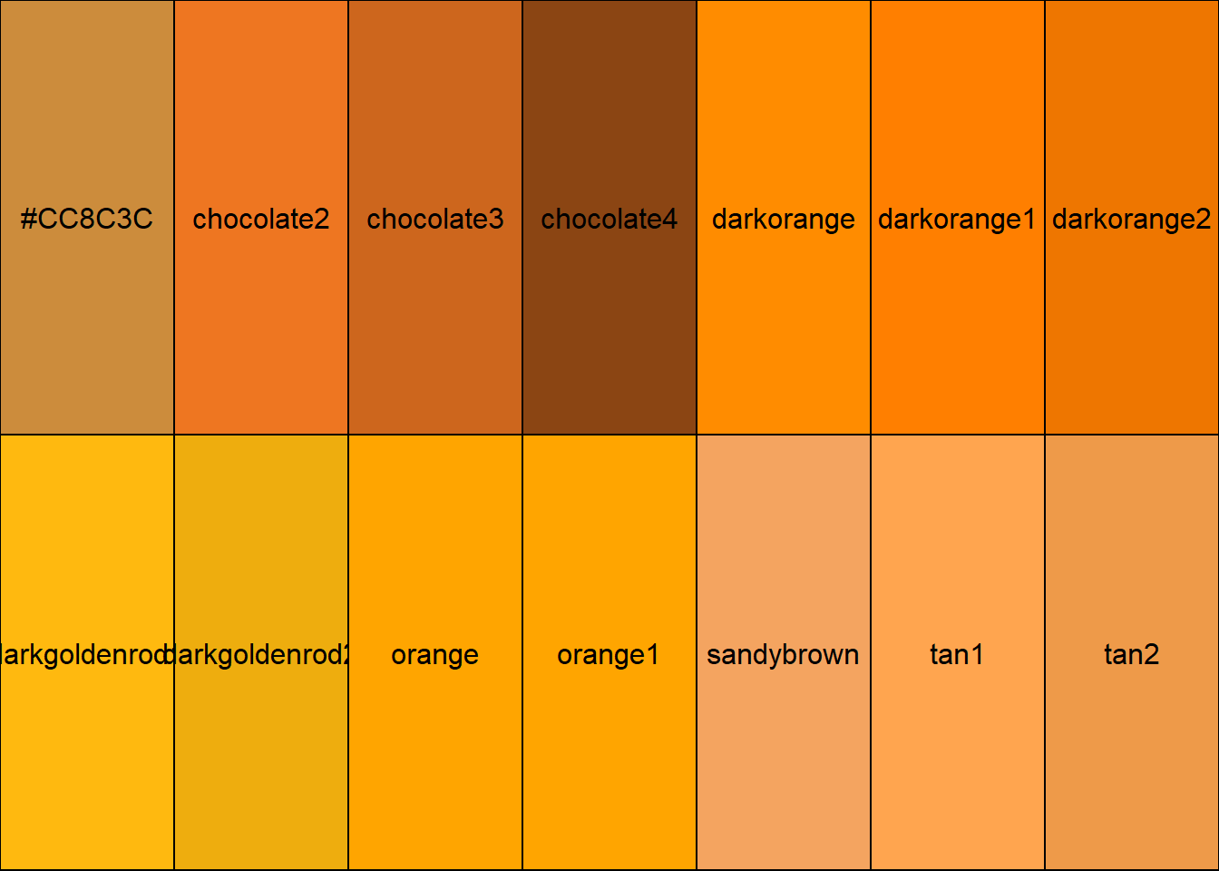
> ##' Find close R colors() to a given color {original by Marius Hofert)
> ##' using Euclidean norm in (HSV / RGB / ...) color space
> nearRcolor <- function(rgb, cSpace = c("hsv", "rgb255", "Luv", "Lab"),
+                        dist = switch(cSpace, "hsv" = 0.10, "rgb255" = 30,
+                        "Luv" = 15, "Lab" = 12))
+ {
+     if(is.character(rgb)) rgb <- col2rgb(rgb)
+     stopifnot(length(rgb <- as.vector(rgb)) == 3)
+     Rcol <- col2rgb(.cc <- colors())
+     uniqC <- !duplicated(t(Rcol)) # gray9 == grey9 (etc)
+     Rcol <- Rcol[, uniqC] ; .cc <- .cc[uniqC]
+     cSpace <- match.arg(cSpace)
+     convRGB2 <- function(Rgb, to)
+         t(convertColor(t(Rgb), from="sRGB", to=to, scale.in=255))
+     ## the transformation,  rgb{0..255} --> cSpace :
+     TransF <- switch(cSpace,
+                      "rgb255" = identity,
+                      "hsv" = rgb2hsv,
+                      "Luv" = function(RGB) convRGB2(RGB, "Luv"),
+                      "Lab" = function(RGB) convRGB2(RGB, "Lab"))
+     d <- sqrt(colSums((TransF(Rcol) - as.vector(TransF(rgb)))^2))
+     iS <- sort.list(d[near <- d <= dist])# sorted: closest first
+     setNames(.cc[near][iS], format(zapsmall(d[near][iS]), digits=3))
+ }

> nearRcolor(col2rgb("tan2"), "rgb")
         0.0         21.1         25.8         29.5
      "tan2"       "tan1" "sandybrown"    "sienna1"

> nearRcolor(col2rgb("tan2"), "hsv")
      0.0000       0.0410       0.0618       0.0638       0.0667       0.0766
      "tan2"    "sienna2"     "coral2"    "tomato2"       "tan1"      "coral"
      0.0778       0.0900       0.0912       0.0918
   "sienna1" "sandybrown"     "coral1"     "tomato"

> nearRcolor(col2rgb("tan2"), "Luv")
        0.00         7.42         7.48        12.41        13.69
      "tan2"       "tan1" "sandybrown"    "orange3"    "orange2"

> nearRcolor(col2rgb("tan2"), "Lab")
        0.00         5.56         8.08        11.31
      "tan2"       "tan1" "sandybrown"       "peru"

> nearRcolor("#334455")
         0.0867
"darkslategray"

> ## Now, consider choosing a color by looking in the
> ## neighborhood of one you know :
>
> plotCol(nearRcolor("deepskyblue", "rgb", dist=50))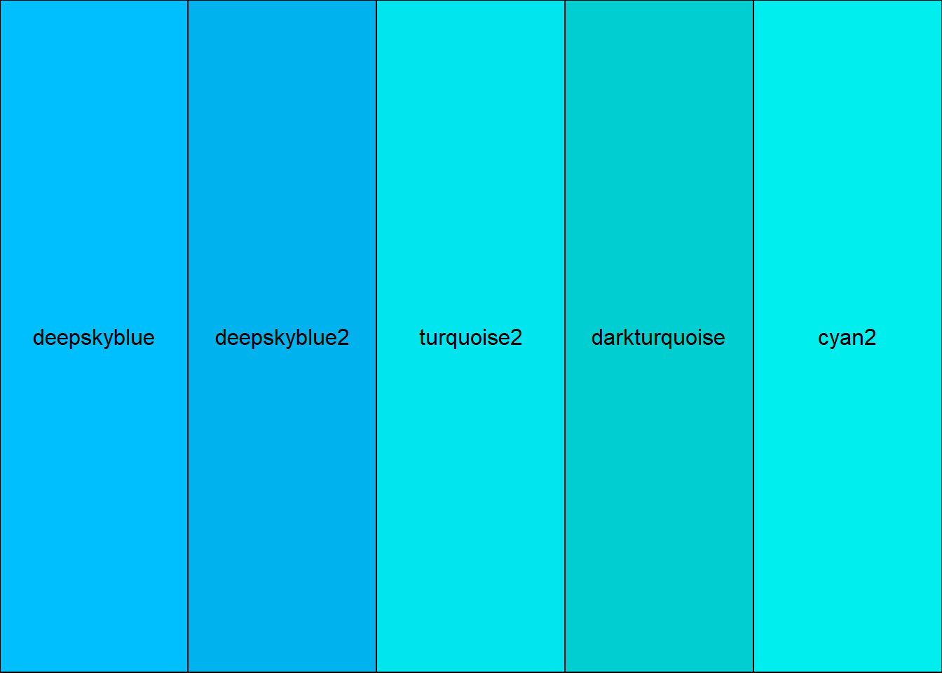
> plotCol(nearRcolor("deepskyblue", dist=.1))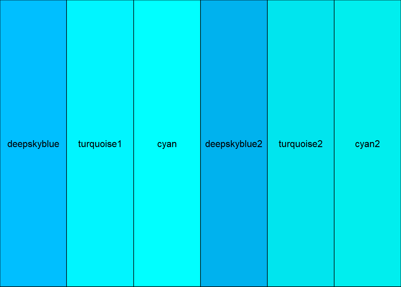
> plotCol(nearRcolor("tomato", "rgb", dist= 50), nrow=3)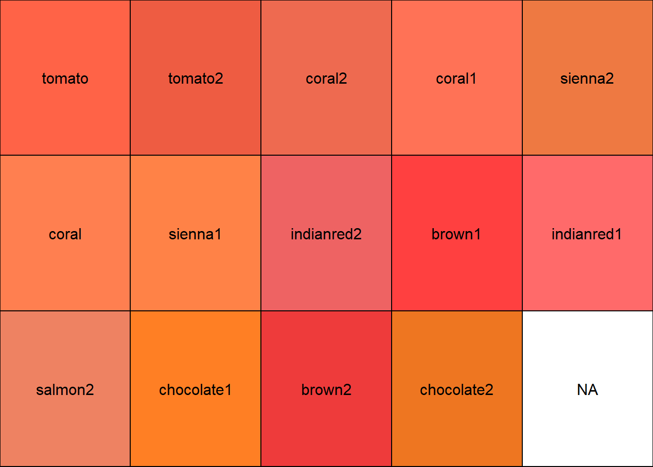
> plotCol(nearRcolor("tomato", "hsv", dist=.12), nrow=3)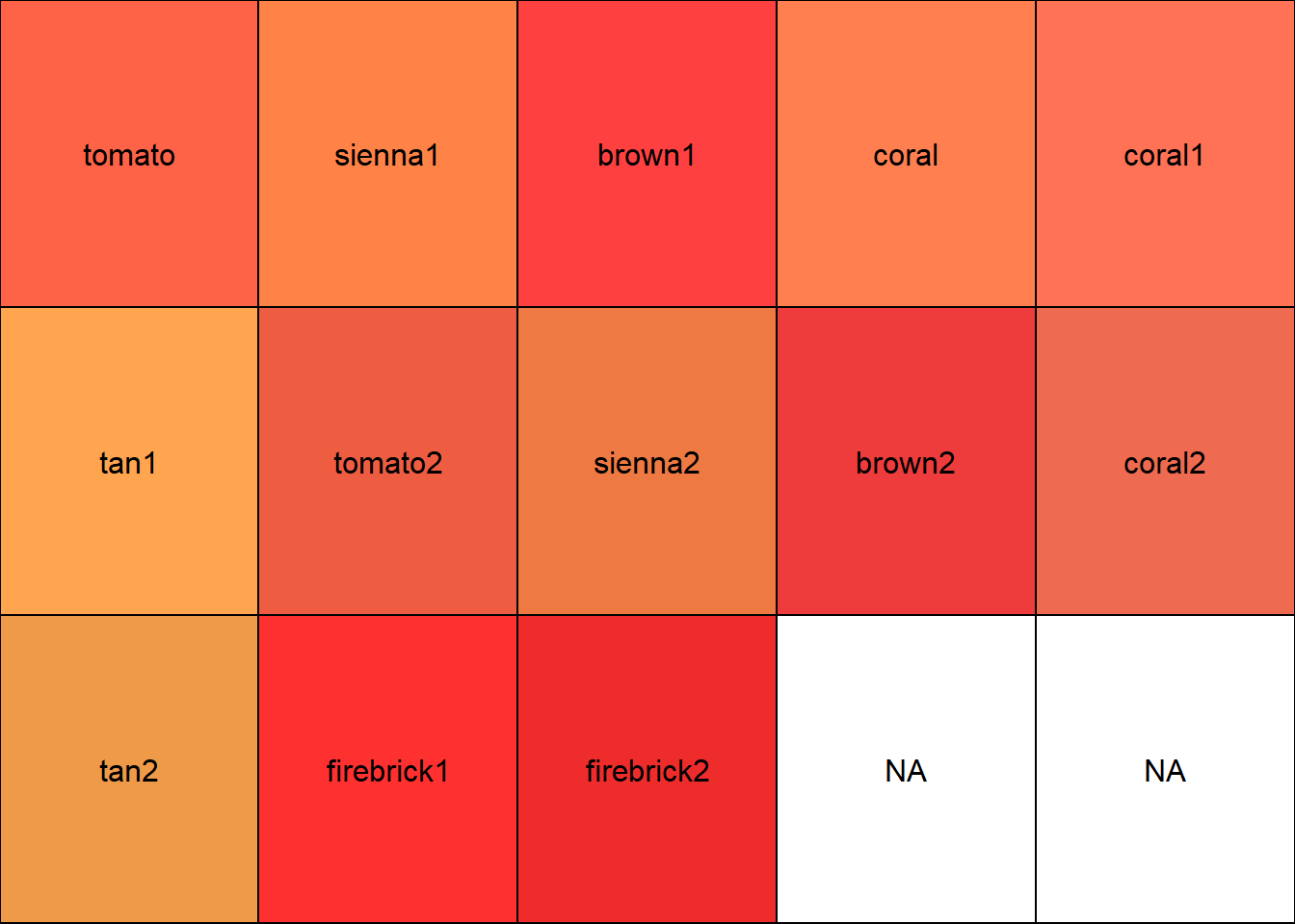
> plotCol(nearRcolor("tomato", "Luv", dist= 25), nrow=3)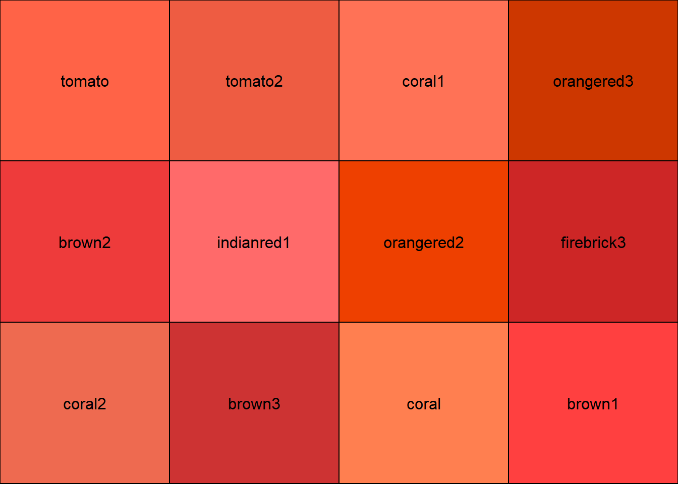
> plotCol(nearRcolor("tomato", "Lab", dist= 18), nrow=3)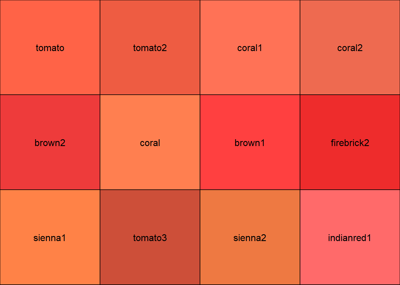
Grid
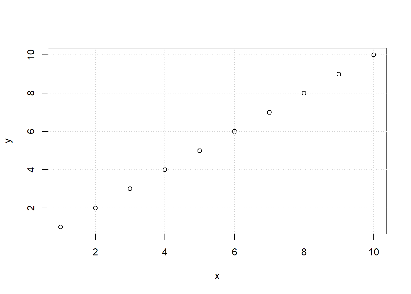
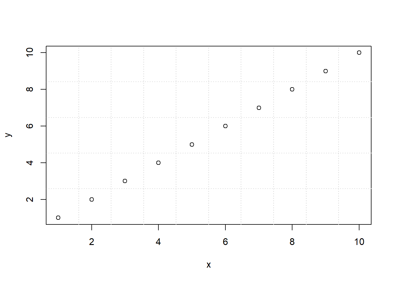
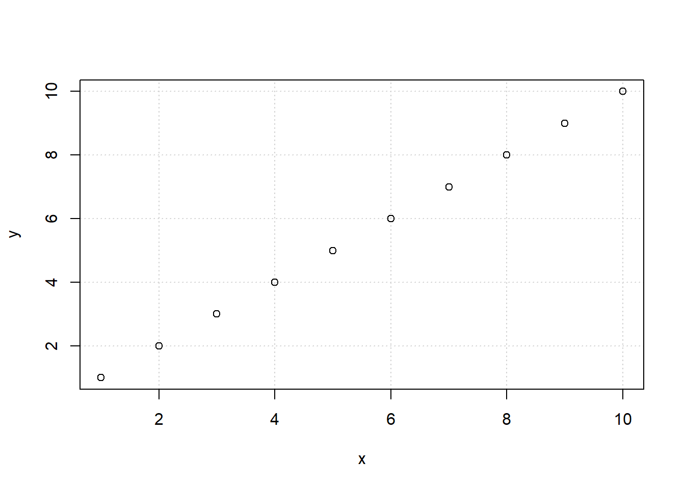
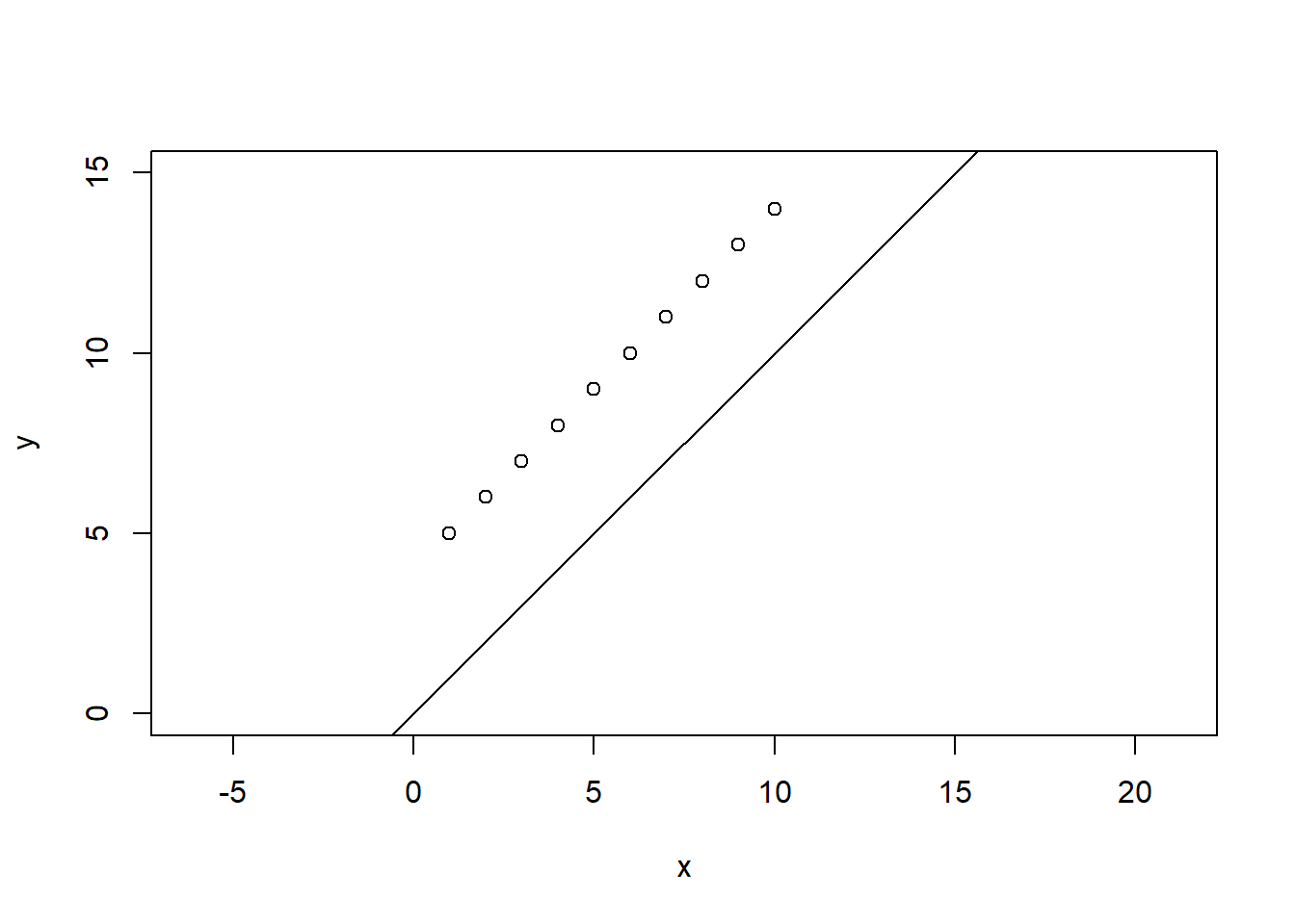
Grid lines should appear behind plot. You can apply panel.first = grid().
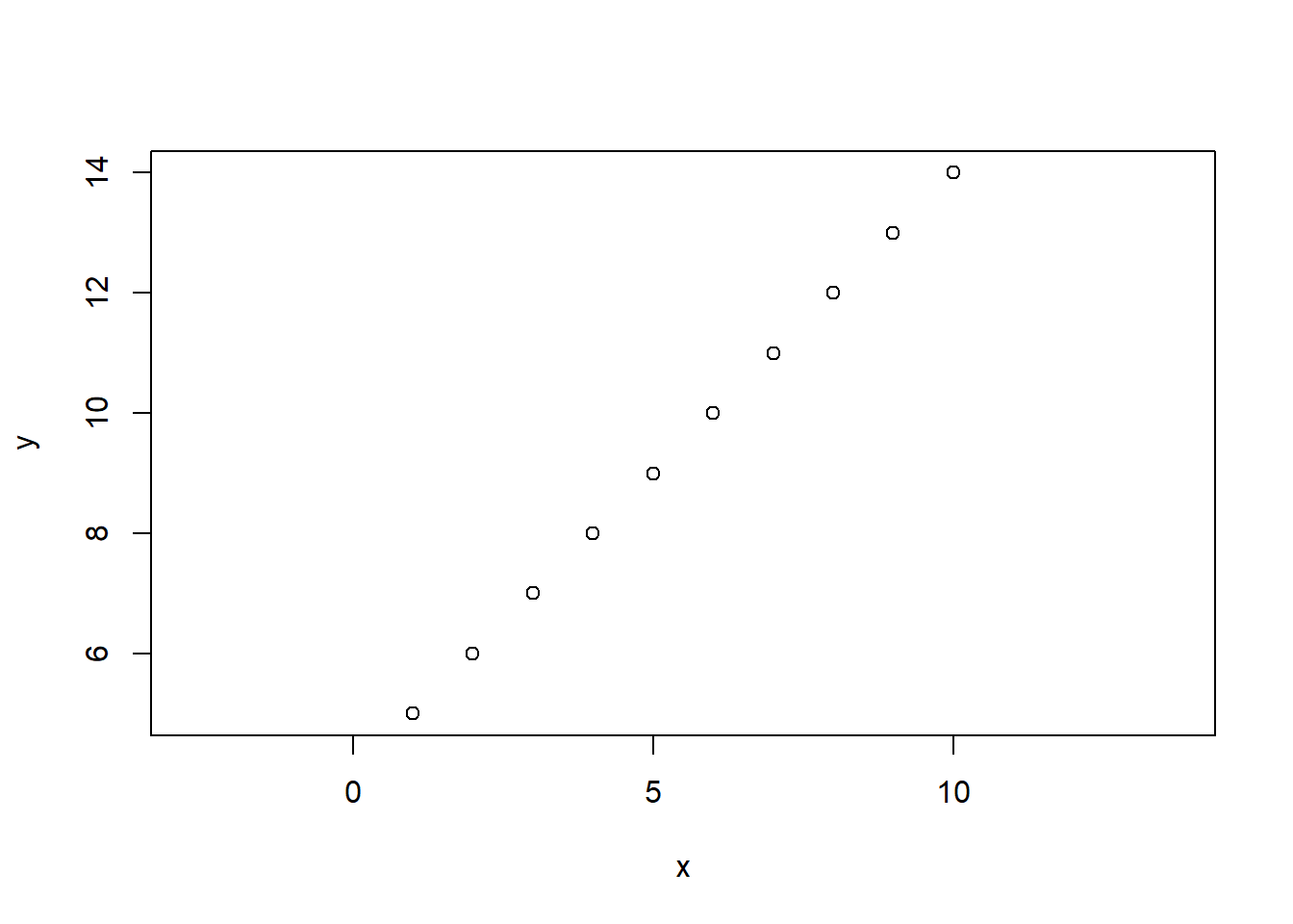
Aspect
asp
Legend
At least, x coordinate x and legend text legend is necessary.
Position
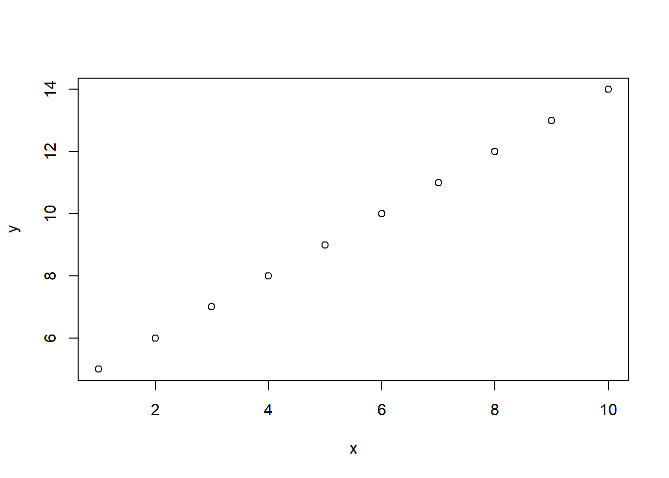
The legend position is specified by x and y coordinates. The reference point is top-left of legend box.
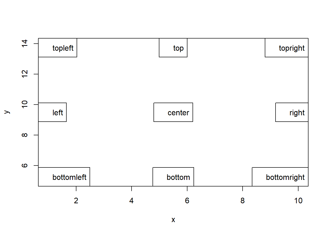
Instead of specific coordinates, keyword can be used. They are intuitive and easy to understand.
plot(x, y, type = "n")
legend("bottomright", legend = "bottomright")
legend("bottom", legend = "bottom")
legend("bottomleft", legend = "bottomleft")
legend("left", legend = "left")
legend("topleft", legend = "topleft")
legend("top", legend = "top")
legend("topright", legend = "topright")
legend("right", legend = "right")
legend("center", legend = "center")